Lecture 7: Data Wrangling II

Adam Altmejd

adam.altmejd@su.se

The Institute for Evaluation of Labour Market and Education Policy (IFAU)

2026-05-05

Today

• Joins / merges
• Reshaping wide <-> long
• Manipulating strings and date time objects
• Applying functions to vectors

Lecture 6 established the core data.table grammar and covered ordinary grouped summaries and grouped transformations. Lecture 7 builds on that foundation by focusing on data table operations restructuring our data.

Lecture 6 gave us the basic grammar

• DT[i, j] to subset and compute
• add by= to summarize and transform by group
• Today we focus on structure: join and reshape
• We will also talk about how to manipulate the data content: strings, regex, and dates

The main shift today is that the data structure becomes less forgiving: rows may need to be ordered within units, keys must identify the right thing, and reshaping can hide missing combinations.

Joining

• Joining

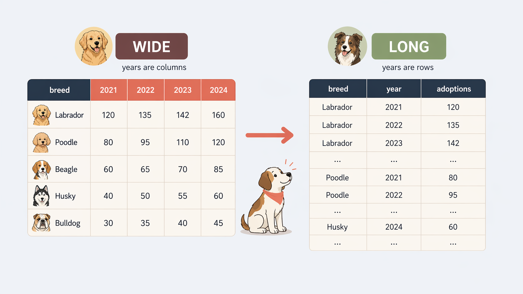
• Reshaping

• Manipulating Strings

• Manipulating Dates and Timestamps

• Iteration

• Extra: More on strings and dates

• Extra: DT non-equi joins and rolling joins

Joining: matching rows across tables

• Two tables share one or more key columns
• A join uses those keys to line up matching rows
• The usual goal is to add columns from one table to another

Joining and merging are the same core idea in this course: combine tables by matching identifiers. The syntax matters, but the structural question matters more. What counts as the key, and what should happen when no match exists?

SQL join types

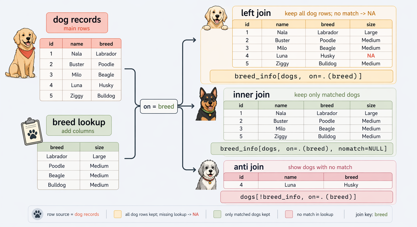
Inner Join: Keep only rows with matching keys in both tables

Left (outer) join: Keep left table, add matches from the right

Full outer join: Keep all rows from both tables

Anti join: Keep rows from left table that have no match in the right

Even outside SQL, these names are useful shorthand. They describe what should happen to the row count and to unmatched observations. The diagram also previews the data.table rule that the object inside the brackets is the row source you keep. Full outer joins are useful for reconciliation tasks, but anti joins are usually the sharper first diagnostic because they isolate exactly which rows failed to match.

The right (outer) join instead keeps the right table, adding matches from the left. But it is rarely used and it is usually better to just swap table places and do a left join.

Primary key vs foreign key

• A (primary) key: uniquely identifies rows
• A foreign key: another table’s primary key
• breed_info$breed should be unique
• dogs$breed is allowed to repeat

This vocabulary clarifies what kind of duplication is normal and what kind is dangerous. Repeated foreign keys are ordinary. Repeated primary keys are often a join bug waiting to happen.

Most join bugs are key bugs

• A join matches rows using key columns
• If the key is wrong, the join is wrong
• If a key is duplicated unexpectedly, rows can multiply
• If keys do not match, rows can silently pick up NA

Joins are mainly data-structure problems not syntax problems. The first question should be about keys and units of observation, not about which join verb to type.

Joining in data.table

data.table has two alternatives:

• merge(x, y, by = "key")
• Y[X, on = "key"] more efficient, allows calculations during join
  • breed_info[dogs, on = .(breed)] is like the SQL command:
  • dogs LEFT JOIN breed_info ON breed

This is the data.table join rule worth memorising: the object inside the brackets determines the rows you keep. Here we keep the dog inventory rows and add matching breed information from breed_info.

Left join: unmatched foreign keys get missing values

breed_info[dogs, on = .(breed)] |>
  _[, .(dog_id, name, breed, avg_life_exp, origin)]

     dog_id     name              breed avg_life_exp         origin
     <char>   <char>             <char>        <num>         <char>
  1:   0013    Buddy Labrador Retriever         11.0         Canada
  2:   3382     Lucy    German Shepherd         11.0        Germany
  3:   4200      Max   Golden Retriever         11.0       Scotland
 ---                                                               
168:   8857    Snowy              Corgi           NA           <NA>
169:   0126 Leo King            Whippet         13.5 United Kingdom
170:   8159      Tut            Whippet         13.5 United Kingdom

This is a crucial interpretation habit. Missing values after a join often mean “no key match”, not “true missing information in the source table”. Those are different diagnoses and need different fixes.

Left join with merge syntax: merge(dogs, breed_info, by = "breed", all.x = TRUE, sort = FALSE)

Inner join: unmatched rows are dropped

breed_info[dogs, on = .(breed), nomatch = NULL] |>
  _[, .(dog_id, name, breed, avg_life_exp, origin)]

     dog_id     name              breed avg_life_exp         origin
     <char>   <char>             <char>        <num>         <char>
  1:   0013    Buddy Labrador Retriever         11.0         Canada
  2:   3382     Lucy    German Shepherd         11.0        Germany
  3:   4200      Max   Golden Retriever         11.0       Scotland
 ---                                                               
145:   8430      Mop            Whippet         13.5 United Kingdom
146:   0126 Leo King            Whippet         13.5 United Kingdom
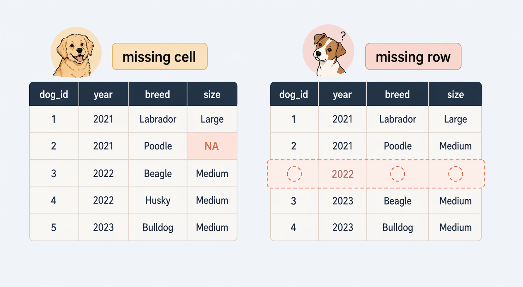
147:   8159      Tut            Whippet         13.5 United Kingdom

The difference is conceptual: do you want to preserve the main table and flag failures, or do you want to drop failures immediately?

Inner join with merge syntax: merge(dogs, breed_info, by = "breed", all = FALSE, sort = FALSE). all = FALSE is the default, but it is good to be explicit about the intended join type.

Anti join: list failed matches

dogs[!breed_info, on = .(breed), .(dog_id, breed)]

    dog_id               breed
    <char>              <char>
 1:   1372 Jack Russel Terrier
 2:   2932 Jack Russel Terrier
 3:   6388 Jack Russel Terrier
---                           
21:   5771               Corgi
22:   1742               Corgi
23:   8857               Corgi

This is essentially an anti-join style diagnostic: show the rows from dogs that did not find a match in breed_info. It is often a much better debugging surface than staring at a large joined table full of NA.

Check the key before trusting the join

Keys should not have duplicates:

anyDuplicated(breed_info, by = "breed")

[1] 0

anyDuplicated(events, by = c("dog_id", "event_time"))

[1] 0

Or missing values:

dogs[, .(missing_breed = sum(is.na(breed)))]

   missing_breed
           <int>
1:             0

events[, .(
  NA_dog_id = sum(is.na(dog_id)),
  NA_event_time = sum(is.na(event_time))
)]

   NA_dog_id NA_event_time
       <int>         <int>
1:         0             0

Duplicate keys can explode the row count

bad_lookup <- rbind(
  breed_info[breed == "Labrador Retriever"],
  breed_info[breed == "Labrador Retriever"]
)

nrow(dogs[breed == "Labrador Retriever"])

[1] 6

nrow(bad_lookup[
  dogs[breed == "Labrador Retriever"],
  on = .(breed),
  allow.cartesian = TRUE
])

[1] 12

This is a deliberately broken lookup table. The dog inventory contains one row per dog, but the duplicated lookup table turns each Labrador row into two rows. Thankfully, data.table refuses duplicate key joins by default, which is why we needed to set allow.cartesian = TRUE.

Joining tables with different units of observation

nrow(dogs)

[1] 170

nrow(sales[dogs, on = .(breed), allow.cartesian = TRUE])

[1] 7155

• dogs has one row per dog
• sales has many rows per breed over time
• Problem is that the tables do not share the same unit of observation

Build a lookup table at the right unit

sales_by_breed <- sales[,
  .(
    sales_n = .N,
    mean_sale_price = round(mean(price_usd), 1),
    last_sale = max(date)
  ),
  by = breed
]

sales_by_breed

                 breed sales_n mean_sale_price  last_sale
                <char>   <int>           <num>     <IDat>
 1:  Poodle (Standard)     143           658.3 2024-12-12
 2: Labrador Retriever      94           551.6 2024-11-28
 3:                Pug     115           653.2 2024-12-23
---                                                      
 8:          Dachshund      89           360.8 2024-12-22
 9:             Beagle      91           362.8 2024-12-14
10:   Golden Retriever      87           561.1 2024-12-20

This is the fix: decide what information should be attached to each dog, then aggregate the sales table to exactly that unit. Once the sales data become one row per breed, they can behave like a lookup table.

Validate the lookup before you join

anyDuplicated(sales_by_breed, by = "breed")

[1] 0

nrow(sales_by_breed)

[1] 10

This is the minimum validation before the repaired join. The lookup key should now be unique. A quick row count also helps with interpretation: the table is now a summary over breeds, not a transaction-level sales table.

Join again and inspect what is still unmatched

dogs_sales <- sales_by_breed[dogs, on = .(breed)]

nrow(dogs_sales)

[1] 170

dogs_sales[is.na(mean_sale_price), unique(breed)]

 [1] "Bulldog"                  "Boxer"                    "Bull Terrier"            
 [4] "Dalmatian"                "Whippet"                  "Irish Setter"            
 [7] "Jack Russel Terrier"      "Boston Terrier"           "Corgi"                   
[10] "Irish Wolfhound"          "Chesapeake Bay Retriever" "Afghan Hound"            

Now the row count is back where it should be: one row per dog. That does not mean the join is perfect, though. Unmatched breeds still need inspection, because they may reflect coverage limits in the sales data rather than random missingness.

Composite keys are common in event logs

event_timing <- events[, .(
  dog_id,
  event_time,
  event_type,
  event_date
)]

event_staff <- events[, .(
  dog_id,
  event_time,
  shelter_name,
  staff_id
)]

event_staff[event_timing, on = .(dog_id, event_time)][1:6]

   dog_id          event_time           shelter_name staff_id event_type event_date
   <char>              <POSc>                 <char>   <char>     <char>     <IDat>
1:   0013 2023-01-15 08:42:00     Happy Paws Shelter      A12     intake 2023-01-15
2:   0013 2023-03-20 23:40:00     Happy Paws Shelter      B07    adopted 2023-03-20
3:   3382 2023-02-10 09:05:00       City Animal Care      A12     intake 2023-02-10
4:   3382 2023-02-13 14:30:00       City Animal Care      V01  vet_check 2023-02-13
5:   3382 2023-04-01 11:30:00       City Animal Care      C03    adopted 2023-04-01
6:   4200 2023-03-05 10:15:00 Willow Creek Adoptions      A08     intake 2023-03-05

This example is intentionally simple because the structure matters more than the novelty. One dog can have several events, so dog_id alone is not enough. The event time is part of the identity of the observation.

i. lets data.table compute during the join

dogs_join <- copy(dogs)

dogs_join[breed_info, on = .(breed), avg_years_left := i.avg_life_exp - age]

dogs_join[1:5, .(dog_id, breed, age, avg_years_left)]

   dog_id              breed   age avg_years_left
   <char>             <char> <int>          <num>
1:   0013 Labrador Retriever     5            6.0
2:   3382    German Shepherd     3            8.0
3:   4200   Golden Retriever     7            4.0
4:   6152            Bulldog     4            5.0
5:   8186             Beagle     6            6.5

The i. prefix refers to columns from the incoming table (the one in i), so the join can directly create a derived column without a separate intermediate object. Similarly, we can use x. to refer to columns from the outer table (DT[]).

Join diagnostics should be routine

• Compare row counts before and after the join
• Check duplicates in the lookup key
• Inspect unmatched rows explicitly
• Re-state the intended unit of observation

These checks are quick and they scale. The habit matters more than memorising a specific join taxonomy.

Detect missing combinations: skeleton + anti-join

events[dog_id %in% c("0013", "3382"),
  .(dog_id, event_time, event_type)]

   dog_id          event_time event_type
   <char>              <POSc>     <char>
1:   0013 2023-01-15 08:42:00     intake
2:   0013 2023-03-20 23:40:00    adopted
3:   3382 2023-02-10 09:05:00     intake
4:   3382 2023-02-13 14:30:00  vet_check
5:   3382 2023-04-01 11:30:00    adopted

skeleton <- CJ(
  dog_id = unique(events$dog_id),
  event_type = c("intake", "vet_check", "adopted")
)
skeleton[!events, on = .(dog_id, event_type)][dog_id %in% c("0013", "3382")]

Key: <dog_id, event_type>
   dog_id event_type
   <char>     <char>
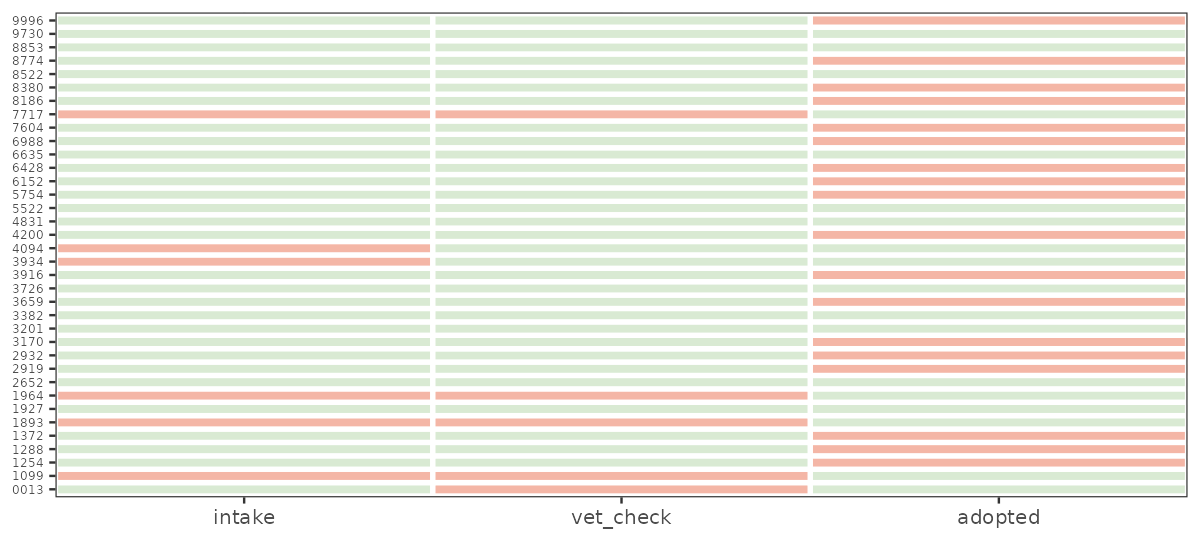
1:   0013  vet_check

• CJ() cross-joins the levels you expected to see
• Anti-join data against the skeleton: what’s left is missing

The pattern is: state what should exist, then ask what’s actually present. The diagnostic is the difference. Much more reliable than visually scanning a table for gaps.

Alternative: A plot can reveal gaps

combination_grid <- events[skeleton, on = .(dog_id, event_type)]
combination_grid[, present := !is.na(event_time)]
combination_grid[, event_type := factor(event_type, levels = c("intake", "vet_check", "adopted"))]
missing_combo_plot <- ggplot(
  combination_grid,
  aes(x = event_type, y = dog_id, fill = present)
) +
  geom_tile(color = "white", linewidth = 1.2) +
  scale_fill_manual(values = c("TRUE" = "#d9ead3", "FALSE" = "#f4b6a6")) +
  scale_x_discrete(expand = c(0, 0)) +
  labs(x = NULL, y = NULL) +
  theme(legend.position = "none",
        axis.text.y = element_text(size = 6))

A quick plot makes the gap obvious (cont.)

This is the same expected-combinations idea as the anti-join, but drawn as a grid. The missing vet_check row for dog 3382 becomes visible immediately.

Reshaping

• Joining

• Reshaping

• Manipulating Strings

• Manipulating Dates and Timestamps

• Iteration

• Extra: More on strings and dates

• Extra: DT non-equi joins and rolling joins

One data set, two shapes

Pick shape by use case

• Wide is convenient for:
  • reading side-by-side and comparing values directly
  • joining the result onto a per-unit table
• Long is convenient for:
  • grouping or summarising by the “variable” itself
  • plotting with ggplot (one column per aesthetic: x, y, colour)
  • adding a new variable without changing the schema

The shape is not “more correct” or “less correct” — it depends on the next operation. A common pipeline is wide-for-reading, long-for-computing, then back to wide for the final output.

Reshaping in data.table

Base R has reshape() but it is clunky. data.table has two more intuitive (and much faster) functions:

• dcast() for long → wide
• melt() for wide → long

dcast(): long → wide

events_long <- events[, .N, by = .(event_date, event_type)]
events_long

    event_date event_type     N
        <IDat>     <char> <int>
 1: 2023-01-15     intake     1
 2: 2023-03-20    adopted     1
 3: 2023-02-10     intake     1
---                            
73: 2023-09-14     intake     1
74: 2023-09-16  vet_check     1
75: 2024-01-08  vet_check     1

dcast(): long → wide

wide_events <- dcast(
  events_long, # long input
  event_date ~ event_type, # rows ~ new columns
  value.var = "N", # what fills each cell
  fill = 0 # default for empty cells
)
wide_events[1:2]

Key: <event_date>
   event_date adopted intake vet_check
       <IDat>   <int>  <int>     <int>
1: 2023-01-15       0      1         0
2: 2023-02-10       0      1         0

• Left of ~ stays as rows
• Right of ~ becomes new column names
• value.var says which column’s values fill the cells

The formula is the heart of dcast: “rows on the left, new columns on the right”. Without fill = 0, missing combinations come out as NA — usually not what you want when the underlying value is a count.

The data.table vignette on reshaping is a good place to learn more.

When cells are not unique, dcast aggregates

breed_events <- events[dogs, on = "dog_id", nomatch = NULL]
dcast(breed_events, breed ~ event_type, fun.aggregate = length, value.var = "dog_id")[1:3]

Key: <breed>
           breed adopted intake vet_check
          <char>   <int>  <int>     <int>
1:        Beagle       1      2         2
2: Border Collie       1      1         1
3:         Boxer       3      4         4

• Many events share each breed × event_type combination
• A cell can only hold one value, so dcast must aggregate
• Default is length with a warning; better to say what you mean
  • Pass fun.aggregate explicitly: length, sum, mean, min, max

If more than one source row maps to the same output cell, dcast cannot produce a single value without aggregating. Explicit beats implicit — say what you want the cell to contain rather than relying on the default.

melt(): wide → long

long_events <- melt(
  wide_events,
  id.vars = "event_date", # columns to keep as-is
  variable.name = "event_type", # name for old column names
  value.name = "N" # name for old cell values
)
long_events

     event_date event_type     N
         <IDat>     <fctr> <int>
  1: 2023-01-15    adopted     0
  2: 2023-02-10    adopted     0
  3: 2023-02-13    adopted     0
 ---                            
205: 2024-03-30  vet_check     1
206: 2024-04-05  vet_check     0
207: 2024-04-08  vet_check     1

• id.vars are the columns that identify a row
• All other columns get stacked into one

Every column not in id.vars is treated as a measurement. Names go into one new column, values into another. The result has more rows and fewer columns — same content, with categories now living as values rather than as a schema.

Why long form pays off

long_events[, .(total = sum(N)), by = event_type]

   event_type total
       <fctr> <int>
1:    adopted    18
2:     intake    30
3:  vet_check    35

• Group by event_type directly
  • In wide form you’d repeat the calculation for each column
• ggplot() wants the same shape: one column per aesthetic
• melt() first often simplifies summary and plotting

A telling sign that you need long form: you are about to write three almost-identical calls, one per column. That is a workflow pushing you toward melt.

Example: A missing row can be hard to notice

A missing cell is an NA value — usually visible in the output. A missing row is an entire expected combination that is absent — invisible unless you build a list of what you expected to see.

Manipulating Strings

• Joining

• Reshaping

• Manipulating Strings

• Manipulating Dates and Timestamps

• Iteration

• Extra: More on strings and dates

• Extra: DT non-equi joins and rolling joins

String = character vector

• Each element is text wrapped in quotes
• Most string functions apply to each element

typeof(c("Buddy", "Lucy"))

[1] "character"

length(c("Buddy", "Lucy"))

[1] 2

nchar(c("Buddy", "Lucy"))

[1] 5 4

Strings in R are character vectors. Operations apply elementwise, which is why they slot into data.table columns directly without an explicit loop.

String problems show up everywhere

• Inconsistent case and whitespace: "Corgi", " corgi", "CORGI "
• Typos that drift over time: "Russel" vs "Russell"
• The same concept under different labels: "Corgi" vs "Pembroke Welsh Corgi"
• Several variables jammed into one column: "03/20-2023"
• Encoding artifacts on imported data

These are not stylistic concerns. They are joins waiting to break. Almost every string job in a wrangling pipeline traces back to one of these patterns.

Encoding is set at import (recap from L6)

fread(file.path(dog_path, "dog_inventory.csv"))[4:6, .(name, `new owner`)]

      name          new owner
    <char>             <char>
1:   Daisy    Ren\xe9e Dubois
2: Charlie       Kenji Tanaka
3: L\xfana Sof\xeda M\xfcller

• For dogs we need to set: fread(..., encoding = "Latin-1")

dogs[grepl("é|í|ö|å", name), unique(name)][1:5]

[1] "Zoé"    "Léo"    "Chloé"  "Söphie" "Növa"  

• Once imported correctly, treat the column as ordinary text
• Mangled accents usually mean the encoding was wrong at import

Encoding lives at the import boundary. If accents look right just after import, treat the column as plain text from there on.

String problems cause join problems

breed_info[dogs, on = .(breed)][
  is.na(avg_life_exp),
  unique(breed)
]

[1] "Jack Russel Terrier" "Corgi"              

breed_info[, unique(grepv("corgi|jack", breed, ignore.case = TRUE))]

[1] "Jack Russell Terrier" "Pembroke Welsh Corgi"

A breed label that almost matches another breed label still fails the equality test the join uses. The visible symptom is missing values after the join, not a string error.

Case and whitespace

sample <- c("Buddy ", "  lucy", "REX", "  Corgi  ")

tolower() / toupper() standardise case

tolower(sample)

[1] "buddy "    "  lucy"    "rex"       "  corgi  "

trimws() removes leading and trailing whitespace

trimws(sample)

[1] "Buddy" "lucy"  "REX"   "Corgi"

nchar() returns each string’s length

nchar(sample)

[1] 6 6 3 9

A lot of “string cleaning” in practice is just casing differences and stray whitespace. These three functions fix the bulk of “almost equal” string problems before any pattern matching is needed.

Building and slicing strings

paste(a, b, sep = " ") and paste0(a, b) glue vectors elementwise

dogs[1:3, paste(name, "the", breed)]

[1] "Buddy the Labrador Retriever" "Lucy the German Shepherd"    
[3] "Max the Golden Retriever"    

sprintf("%s ... %d", ...) for templated output: - %s strings, %d integers, %f doubles

dogs[1:3, sprintf("%s (%d years old)", name, age)]

[1] "Buddy (5 years old)" "Lucy (3 years old)"  "Max (7 years old)"  

substr(x, start, stop) extracts characters by position

dogs[1:3, substr(name, 1, 3)]

[1] "Bud" "Luc" "Max"

Position-based extraction is fine when the format is rigid — for example, the first three letters of a fixed-width code. When the position varies, that is where regex enters.

Regex: a pattern language

When equality is not enough:

• Find every breed starting with “Lab”
• Find typos: “Russel” or “Russell”
• Split "03/20-2023" on either / or -

A regular expression (regex) describes a pattern of text:

• Built into grepl(), sub(), gsub(), tstrsplit(), …
• Same syntax across R, Python, JavaScript, grep, sed
• A plain string is already a valid regex — "Corgi" matches "Corgi"
• The power comes from metacharacters: ^, $, ., *, +, [...], |

Regex pays back the small learning curve many times over. Once these patterns are readable, parsing odd column shapes stops being a custom job each time.

Reading a regex

^[A-Z][a-z]+ Russel+$ reads left-to-right as:

1. ^ — start of string
2. [A-Z] — one uppercase letter
3. [a-z]+ — one or more lowercase letters
4. Russe — a space, then literal text
5. l+ — one or more ls (matches “Russel” and “Russell”)
6. $ — end of string

Reading a regex

Symbol	Meaning
[abc]	one of a, b, c
[a-z]	any lowercase letter
.	any single character
* / + / ?	zero+, one+, or zero-or-one of the previous
\\s / \\d	whitespace / digit
^ / $	start / end of string
|	OR — either pattern

\ is special in R strings, so regex backslashes are doubled (escaped): \\s, \\d, \\..

Detect with grepl

# literal: contains "Corgi"
dogs[grepl("Corgi", breed), unique(breed)]

[1] "Corgi"

# alternation: either "Russel" or "Corgi"
dogs[grepl("Russel|Corgi", breed), unique(breed)]

[1] "Jack Russel Terrier" "Corgi"              

# case-insensitive
dogs[grepl("corgi", breed, ignore.case = TRUE), unique(breed)]

[1] "Corgi"

• grepl(pattern, x) returns TRUE/FALSE per element
• grepv() returns the matching values

Plain text is the simplest possible “pattern”: it just matches itself. Alternation with | checks several variants in one call. ignore.case = TRUE is the regex-aware shortcut for “lowercase both sides before matching”. grepv() is shorthand for grep(pattern, x, value = TRUE).

Anchors

^ matches the start of the string

breed_info[, grepv("^Lab", breed)]

[1] "Labrador Retriever"

$ matches the end of the string

breed_info[, grepv("ver$", breed)]

[1] "Labrador Retriever"       "Golden Retriever"         "Chesapeake Bay Retriever"

Anchors and quantifiers cover the bulk of pattern-matching needs in data wrangling. Collapsing repeated whitespace is a common preprocessing step on free-text fields.

Replace with sub and gsub

dogs[, breed := gsub("Rus+el+", "Russell", breed)]
dogs[grep("[Cc]orgi", breed), breed := "Pembroke Welsh Corgi"]

breed_info[dogs, on = .(breed)][
  is.na(avg_life_exp),
  unique(breed)
]

character(0)

• sub(pat, repl, x) — replace first match per element
• gsub(pat, repl, x) — replace all matches per element

gsub("\\s+", " ", c("Border  Collie", "Labrador   Retriever"))

[1] "Border Collie"      "Labrador Retriever"

• \\s for a whitespace character
• + for one or more of the preceding character

Detect, replace, then re-run the join check. Repairing labels in place is much better than pretending the mismatch was random missingness.

Manipulating Dates and Timestamps

• Joining

• Reshaping

• Manipulating Strings

• Manipulating Dates and Timestamps

• Iteration

• Extra: More on strings and dates

• Extra: DT non-equi joins and rolling joins

What is a date object?

• A Date stores a calendar day with no time of day
• Internally it is a number: days since 1970-01-01
• Arithmetic and comparisons work on that number
• Printing formats the number back as a calendar string

d <- as.Date("2024-02-28")

class(d)

[1] "Date"

unclass(d)

[1] 19781

d + 3

[1] "2024-03-02"

d - as.Date("2022-02-28")

Time difference of 730 days

Dates are numbers underneath. That is what makes addition, subtraction, sorting, and grouping behave sensibly. The string we see is just a formatted view of the number.

What is a timestamp object?

• A POSIXct stores an instant in time, accurate to seconds
• Internally it is a number: seconds since 1970-01-01 UTC
• It carries a timezone attribute that controls how it prints

t <- as.POSIXct("2024-03-20 23:40:00", tz = "Europe/Stockholm")

class(t)

[1] "POSIXct" "POSIXt" 

unclass(t)

[1] 1710974400
attr(,"tzone")
[1] "Europe/Stockholm"

format(t, tz = "UTC", usetz = TRUE)

[1] "2024-03-20 22:40:00 UTC"

A timestamp is an instant plus a way of displaying it. The timezone is metadata for the display, not part of the underlying number.

Base R also has POSIXlt, which stores the same instant as a list of components (year, month, day, hour, …). Prefer POSIXct for stored data; POSIXlt is mostly useful when you want direct component access without format().

Date vs data.table::IDate

• IDate is data.table’s calendar-date type — integer-backed, ~half the memory of base R Date
• IDate inherits from Date, so the two are interchangeable in almost all operations
• Date / IDate: day only — no time of day, no timezone
• Don’t record time if you don’t need it — it’s a common source of problems

Picking the right type prevents a common overcomplication. Calendar dates are enough for intake and sale days. POSIXct is needed for events, logs, appointment times — anything where time of day and timezone change the meaning.

data.table also provides ITime for time-of-day (seconds since midnight, no date or timezone). Useful when only the clock time matters — e.g., “events by hour of day across all days”.

Strings that look like dates are not dates

dogs[, sale_date - intake_date]

Error in `-.IDate`:
! can only subtract from "IDate" objects

sapply(dogs[, .(intake_date, sale_date)], class)

$intake_date
[1] "IDate" "Date" 

$sale_date
[1] "character"

The error is the symptom; the class output is the diagnosis. sale_date is still character, so date arithmetic has no sensible type to operate on. Looking like a date and being a date are different things.

Parsing strings into dates

• Same idea for both: tell R the format, get a real type back
• as.IDate(x, format = ...) for calendar dates
• as.POSIXct(x, format = ..., tz = ...) for timestamps
• fread() parses common formats automatically — flag suspect columns and re-parse
• The format string describes the input, not the output

Parsing is a contract: the strings on disk look like X, so R should produce a date or a timestamp. Once that contract is met, every later operation gets simpler.

strptime format codes

Code	Meaning
%Y	year, 4-digit
%y	year, 2-digit
%m	month number
%B	month name
%b	month abbreviated
%d	day of month

Code	Meaning
%H	hour (24h)
%M	minute
%S	second
%F	%Y-%m-%d shortcut
%T	%H:%M:%S shortcut

as.IDate("13 March 2024", format = "%d %B %Y")

[1] "2024-03-13"

R uses the same POSIX codes as most other languages. Once you can read these codes, the format string for any input becomes mechanical to write.

%B and %b depend on the locale — in a non-English session, “March” may not parse.

Parse explicitly when the format is unusual

str(dogs$sale_date)

 chr [1:170] "03/20-2023" "04/01-2023" "06/15-2023" "07/11-2023" "08/02-2023" ...

dogs[, sale_date := as.IDate(sale_date, format = "%m/%d-%Y")]
dogs[1:5, .(dog_id, intake_date, sale_date)]

   dog_id intake_date  sale_date
   <char>      <IDat>     <IDat>
1:   0013  2023-01-15 2023-03-20
2:   3382  2023-02-10 2023-04-01
3:   4200  2023-03-05 2023-06-15
4:   6152  2023-04-20 2023-07-11
5:   8186  2023-05-11 2023-08-02

Non-standard formats need an explicit format string. The format is part of the cleaning contract, not a detail to keep in your head.

Avoid format codes with lubridate

• Function names spell out component order: ymd, mdy, dmy
• ymd_hms("2024-03-20 23:40:00") for timestamps
• Optional tz = argument; otherwise UTC

mdy("03/20-2023")

[1] "2023-03-20"

ymd_hms("2024-03-20 23:40:00", tz = "Europe/Stockholm")

[1] "2024-03-20 23:40:00 CET"

lubridate removes the format-string burden for common cases. The function name encodes the component order, so guessing the format is rarely necessary.

Cheat sheet: https://github.com/rstudio/cheatsheets/blob/main/lubridate.pdf. Fall back to as.IDate(x, format = ...) for genuinely unusual formats or when an IDate is needed directly.

fread() recognises timestamps automatically

ts <- fread(
  file.path(dog_path, "dog_events.csv"),
  colClasses = list(character = "dog_id")
)[dog_id == "0013" & event_type == "adopted", .(dog_id, event_type, event_time)]
ts

   dog_id event_type          event_time
   <char>     <char>              <POSc>
1:   0013    adopted 2023-03-20 23:40:00

class(ts$event_time)

[1] "POSIXct" "POSIXt" 

attr(ts$event_time, "tzone")

[1] "UTC"

Warning! Assumes the timezone is UTC

Automatic parsing is convenient, but it still needs inspection. The CSV here records local Swedish clock time, but the file does not store a timezone — so fread() has to guess on UTC which is wrong.

Assuming the wrong timezone can shift dates

format(ts$event_time, tz = "Europe/Stockholm")

[1] "2023-03-21 00:40:00"

as.POSIXct(ts$event_time, tz = "Europe/Stockholm")

[1] "2023-03-21 00:40:00 CET"

as.IDate(ts$event_time, tz = "Europe/Stockholm")

[1] "2023-03-21"

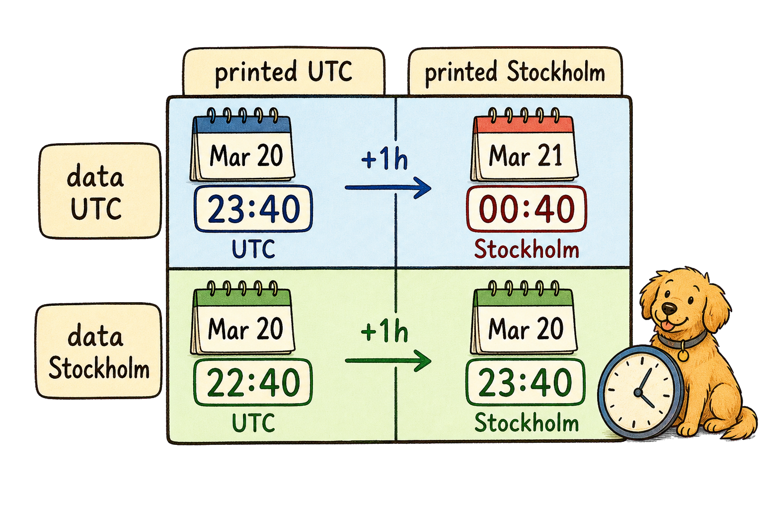
All outputs change time/dates instead of timezone.

The string is identical in both paths. If the timestamp is wrongly treated as UTC, displaying or aggregating it in Swedish time moves it to the next calendar date. Need to read the timestamp as text first, then parse with the correct timezone to get the right instant. Or use lubridate::force_tz() to fix ex post.

Fix: read as text, then parse with the correct timezone

ts_fix <- fread(
  file.path(dog_path, "dog_events.csv"),
  colClasses = list(character = c("dog_id", "event_time"))
)[dog_id == "0013" & event_type == "adopted", .(dog_id, event_type, event_time)]
ts_fix[,
  event_time := as.POSIXct(
    event_time,
    format = "%Y-%m-%d %H:%M:%S",
    tz = "Europe/Stockholm"
  )
]
ts_fix

   dog_id event_type          event_time
   <char>     <char>              <POSc>
1:   0013    adopted 2023-03-20 23:40:00

The timezone comes from metadata or domain knowledge, not from the column itself. Reading the timestamp as text first prevents the parser from silently assigning the wrong instant before the code has a chance to say what the clock time meant.

Better fix from the lubridate package

with_tz(t, "Europe/Stockholm") keeps instant, changes display

with_tz(ts$event_time, "Europe/Stockholm")

[1] "2023-03-21 00:40:00 CET"

force_tz(t, "Europe/Stockholm") keeps time, changes instant

force_tz(ts$event_time, "Europe/Stockholm")

[1] "2023-03-20 23:40:00 CET"

The same input can produce two different timestamps depending on which function you reach for. Choose by asking: did the source already record the right instant, or did it record clock time without a timezone?

Date arithmetic and comparison

dogs[, stay_days := sale_date - intake_date]

dogs[
  !is.na(stay_days),
  .(
    average_stay_days = mean(stay_days),
    longest_stay = max(stay_days)
  )
]

   average_stay_days longest_stay
          <difftime>   <difftime>
1:     87.19403 days     116 days

dogs[sale_date > as.IDate("2024-01-01"), .N]

[1] 42

Subtraction returns a difference in days. Comparison and sorting work the way you expect once the type is right.

Extract date components (with lubridate)

dogs[
  !is.na(sale_date),
  .(
    sale_date,
    year = year(sale_date),
    month = month(sale_date),
    day = mday(sale_date),
    weekday = wday(sale_date)
  )
][1:5]

    sale_date  year month   day weekday
       <IDat> <num> <num> <int>   <num>
1: 2023-03-20  2023     3    20       2
2: 2023-04-01  2023     4     1       7
3: 2023-06-15  2023     6    15       5
4: 2023-07-11  2023     7    11       3
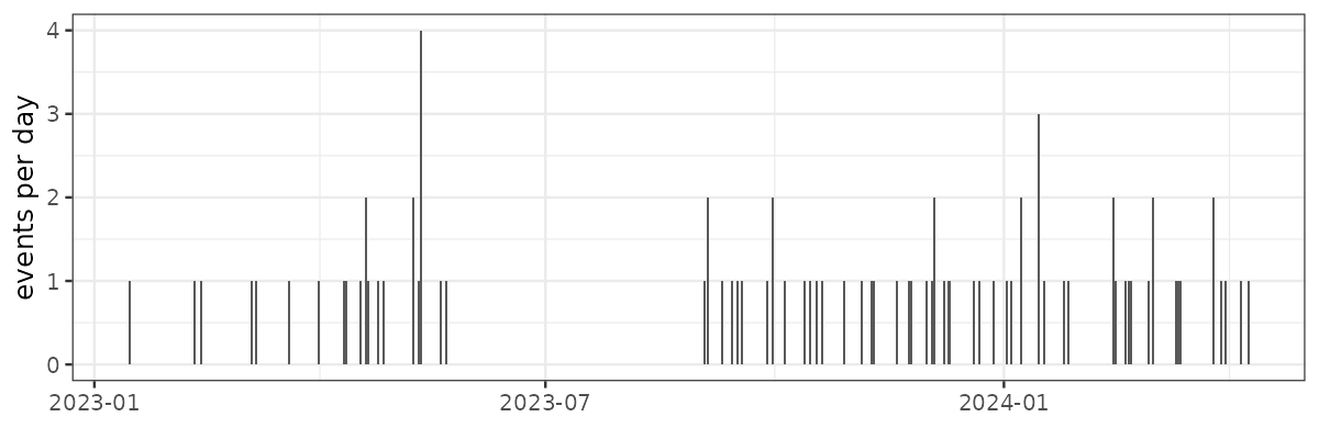
5: 2023-08-02  2023     8     2       4

Component accessors are cleaner than reformatting the date as text and re-parsing the parts. The wday() convention is a footgun: depending on the package and locale defaults, the week may start on Sunday or Monday.

Component accessors year(), month(), mday(), wday(), quarter(), yday() come from lubridate (already loaded) and also work on IDate. wday() returns 1 for Sunday by default — pass week_start = 1 for Monday.

Round dates and month-safe arithmetic (lubridate)

floor_date(as.Date("2024-03-20"), unit = "month")

[1] "2024-03-01"

ceiling_date(as.Date("2024-03-20"), unit = "week")

[1] "2024-03-24"

as.Date("2024-01-31") + months(1) # NA — Feb 31 does not exist

[1] NA

as.Date("2024-01-31") %m+% months(1) # 2024-02-29 — clamps to month end

[1] "2024-02-29"

floor_date() and ceiling_date() truncate or extend a date to a calendar boundary, keeping it as a date — much cleaner than the format(..., "%Y-%m-01") trick. Plain + months(1) is strict: if the target day does not exist (Feb 31), it returns NA. %m+% and %m-% clamp to the last day of the target month, which is usually what you want.

Using floor_date in by= for monthly aggregation

# Aggregate sales by month
dogs[!is.na(sale_date), .N, by = .(month = floor_date(sale_date, "month"))][1:6]

        month     N
       <Date> <int>
1: 2023-03-01     1
2: 2023-04-01     1
3: 2023-06-01     7
4: 2023-07-01     9
5: 2023-08-01    14
6: 2023-09-01    13

Time differences with difftime

t1 <- as.POSIXct("2024-03-20 23:40:00", tz = "Europe/Stockholm")
t2 <- as.POSIXct("2024-03-21 09:15:00", tz = "Europe/Stockholm")

t2 - t1

Time difference of 9.583333 hours

difftime(t2, t1, units = "hours")

Time difference of 9.583333 hours

as.numeric(difftime(t2, t1, units = "hours"))

[1] 9.583333

Subtracting timestamps returns a difftime. The default unit can flip from seconds to minutes to days depending on the gap, which is a quiet source of bugs. Forcing the unit and converting to numeric makes downstream arithmetic predictable.

The default unit chosen by - and by difftime() depends on the magnitude. Pass units = explicitly when the result feeds into arithmetic.

Using dates in diagnostic plots

A count over time graph can reveal missing data that a tabular check would miss.

events[, .N, by = event_date] |>
  ggplot(aes(x = event_date, y = N)) +
  geom_col() +
  labs(x = NULL, y = "events per day")

ggplot allows plots dates, just make sure the type is not character and the x-axis will be scaled appropriately.

Iteration

• Joining

• Reshaping

• Manipulating Strings

• Manipulating Dates and Timestamps

• Iteration

• Extra: More on strings and dates

• Extra: DT non-equi joins and rolling joins

Vectorise or use by before you iterate with loops

• Same summary by group → by=
• Same rule on several columns → .SD
• Same operation across separate files or objects → iterate

data.table already loops for you in the first two cases. Iterate only when the inputs are inherently separate — different files, different objects. The next slides cover the family of R functions that handle that kind of iteration cleanly.

lapply() and relatives

• lapply(x, f) calls f on each element of x — returns a list, one result per input
• Predictable shape: length(input) == length(output)
• The wider family differs in how the output is shaped:
  • sapply(x, f) — simplify to a vector or matrix when possible
  • vapply(x, f, FUN.VALUE) — like sapply with a type contract
  • mapply(f, x, y) — parallel iteration over several vectors
  • apply(M, MARGIN, f) — over rows or columns of a matrix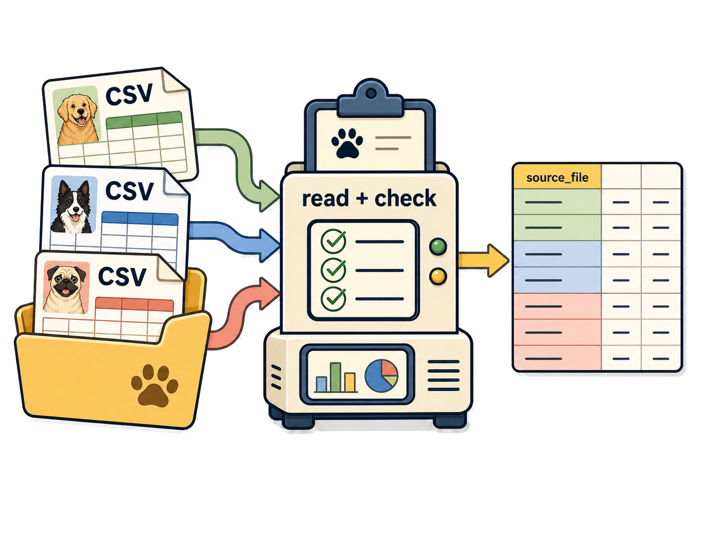

Counting the number of characters in each word

words <- c("Buddy", "Lucy", "Rex")

# list of results
lapply(words, nchar)

[[1]]
[1] 5

[[2]]
[1] 4

[[3]]
[1] 3

# simplified to a named vector
sapply(words, nchar)

Buddy  Lucy   Rex 
    5     4     3 

The whole family applies a function elementwise over a vector or list. They differ mainly in the output shape. For data wrangling we usually want lapply: a predictable list of one result per input pairs cleanly with rbindlist. Prefer lapply over a for loop because the return value is the point — you want one object containing all results, not side effects.

Example: reading many files at once

basename(event_paths)

[1] "city_animal_care_events.csv"       "happy_paws_shelter_events.csv"    
[3] "willow_creek_adoptions_events.csv"

• One CSV per shelter, dropped in a folder
• Read them all with the right types, stacked into one table
• Keep track of which row came from which file

A realistic reason to iterate: the inputs live in separate files, but the same reading logic should apply to all of them. In a project, these files would already exist; here they are written from events_raw in a hidden setup chunk.

Write a reusable reader function

read_dog_events <- function(path) {
  if (!file.exists(path)) {
    warning("File not found, skipping: ", path)
    return(NULL)
  }
  dt <- fread(path, colClasses = list(character = c("dog_id", "event_time")))
  dt[,
    event_time := as.POSIXct(
      event_time,
      format = "%Y-%m-%d %H:%M:%S",
      tz = "Europe/Stockholm"
    )
  ]
  dt[, event_date := as.IDate(event_time, tz = "Europe/Stockholm")]
  dt
}

• Pin down the format quirks: character IDs, Swedish local time
• warning() flags a problem without aborting the batch
• Returning NULL lets rbindlist() skip the file silently

The function captures the rules that a future you, or another student, will otherwise forget by the third script. The missing-file branch uses warning() instead of stop() so a single bad path does not kill a 50-file run; rbindlist() drops NULL list elements automatically.

Workhorse pattern: lapply() + rbindlist(idcol = ...)

event_list <- lapply(event_paths, read_dog_events)
names(event_list) <- basename(event_paths)

all_events <- rbindlist(event_list, idcol = "source_file")
all_events[, .(rows = .N, dogs = uniqueN(dog_id)), by = source_file]

                         source_file  rows  dogs
                              <char> <int> <int>
1:       city_animal_care_events.csv    31    12
2:     happy_paws_shelter_events.csv    27    13
3: willow_creek_adoptions_events.csv    25    11

• lapply() returns one list element per file
• Naming the list lets rbindlist(idcol = ...) keep provenance
• rbindlist silently drops NULL entries
  • A missing file just doesn’t contribute rows

This is the entire multi-file import pattern in three lines. The names on the list become the values in the source_file column, so you can always see which row came from which file. If read_dog_events returned NULL for a missing file, that element is dropped from the bind without complaint — combined with the warning() in the reader, the batch reports the problem and keeps going.

Validation checklist

After every join, reshape, or type change:

• Row count — did it change as expected?
• Key uniqueness — duplicates can explode joins
• Unmatched rows — which ones, and why?
• Missing combinations — anything absent that should exist?
• Types — dates are dates, IDs stayed character

Five fast checks. Done individually they are trivial; done as a habit they catch most of the bugs that survive into reports.

Main takeaways

• Join problems are usually key problems
• Wide vs long is a question about what each row represents — pick the shape that fits the use case
• String and date cleaning are often prerequisites for correct joins
• Keep validating: check row counts, unit of observation, unmatched rows after every join, reshape, or type change
• Wrap repeated logic in a function, then apply it with lapply()

Next lecture: APIs and external data

Extra: More on strings and dates

• Joining

• Reshaping

• Manipulating Strings

• Manipulating Dates and Timestamps

• Iteration

• Extra: More on strings and dates

• Extra: DT non-equi joins and rolling joins

Split with tstrsplit

sale_parts <- dogs[!is.na(sale_date), .(sale_date)]
sale_parts[,
  c("sale_month", "sale_day", "sale_year") := tstrsplit(sale_date, "[/-]")
]

sale_parts[1:5]

    sale_date sale_month sale_day sale_year
       <IDat>     <char>   <char>    <char>
1: 2023-03-20       2023       03        20
2: 2023-04-01       2023       04        01
3: 2023-06-15       2023       06        15
4: 2023-07-11       2023       07        11
5: 2023-08-02       2023       08        02

• [/-] matches either / or - — handles inconsistent delimiters in one pass
• Useful when one column hides several variables
• For dates specifically, parse to a real type instead — that is the next section

The split character itself is a regex, so [/-] handles inconsistent delimiters in a single pass. If the goal is a date, parse it directly rather than keeping the parts as character columns.

stringr offers a more consistent grammar

• All functions start with str_ and take the string first
• str_detect(x, pattern) for grepl
• str_replace_all(x, pattern, replacement) for gsub
• str_to_lower(x), str_squish(x), str_split_fixed(x, sep, n)
• Named vectors handle multiple replacements at once

library(stringr)
dogs[, breed := str_replace_all(breed, c(
    "Russel"  = "Russell",
    "^Corgi$" = "Pembroke Welsh Corgi"
))]

Either toolkit is fine. Function names are more consistent in stringr, and the named-vector form is convenient for batched replacements. The thing to avoid is mixing both inside one project.

ISO 8601 week convention

• Plain “week of the year” is ambiguous — does week 1 start Sun or Mon? Does it start in the old or new year?
• ISO 8601 fixes a convention:
  • weeks run Mon–Sun
  • week 1 is the one containing the year’s first Thursday
• Standard in business, public-health, and official statistics reporting (Eurostat, ECDC, retail) — needed if your data must line up with those sources

ISO week footgun

ISO weeks have their own year. Dec 30, 2024 is ISO week 1 of 2025; pair isoyear() with isoweek(), never year()

dogs[
  !is.na(sale_date),
  .N,
  by = .(
    iso_year = isoyear(sale_date),
    iso_week = isoweek(sale_date)
  )
][order(iso_year, iso_week)][1:8]

   iso_year iso_week     N
      <num>    <num> <int>
1:     2023       12     1
2:     2023       13     1
3:     2023       18     1
4:     2023       19     2
5:     2023       20     1
6:     2023       21     1
7:     2023       22     1
8:     2023       23     2

Extra: DT non-equi joins and rolling joins

• Joining

• Reshaping

• Manipulating Strings

• Manipulating Dates and Timestamps

• Iteration

• Extra: More on strings and dates

• Extra: DT non-equi joins and rolling joins

Non-equi joins: match with inequalities

window <- data.table(start = as.IDate("2023-06-01"), end = as.IDate("2023-06-15"))
sales[window,
  on = .(date >= start, date <= end),
  .(breed, sale_date = x.date, price_usd),
  nomatch = NULL]

                 breed  sale_date price_usd
                <char>     <IDat>     <int>
 1:          Chihuahua 2023-06-08       341
 2:     French Bulldog 2023-06-08       867
 3: Labrador Retriever 2023-06-03       592
---                                        
19:      Border Collie 2023-06-01       486
20:     French Bulldog 2023-06-13      1233
21:             Beagle 2023-06-09       402

• on = accepts <, <=, >, >= instead of ==
• Match: rows where date falls inside the window

Build a small table whose rows are the windows you care about, then join with inequalities. Generalises to report periods, treatment exposure intervals, billing cycles. nomatch = NULL drops query rows that found nothing (inner-join behaviour).

Rolling joins: as-of lookup

sales_lab <- sales[breed == "Labrador Retriever", .(date, price_usd)]
setkey(sales_lab, date)
queries <- data.table(date = as.IDate(c("2023-01-15", "2023-06-15", "2023-12-08")))
sales_lab[queries, on = "date", roll = TRUE]

         date price_usd
       <IDat>     <int>
1: 2023-01-15       618
2: 2023-06-15       592
3: 2023-12-08       587

• For each query date, find the most recent earlier observation
• roll = TRUE carries the last prior value forward; roll = "nearest" picks closest in either direction

Common in time-series work: “what was the value just before this moment?”. data.table walks the sorted key once instead of the manual filter-and-take-latest pattern. The lookup table must be sorted on the rolling column — hence setkey().

Data table magic

Now combine both ideas. Let’s calculate the average price during two months around each sale:

dogs[
  sales[
    dogs[
      !is.na(sale_date),
      .(
        dog_id,
        breed,
        date1 = as.Date(sale_date) %m-% months(2),
        date2 = as.Date(sale_date) %m+% months(2)
      )
    ],
    on = c("breed", "date >= date1", "date < date2"),
    by = .EACHI,
    .(dog_id, mean_price = mean(price_usd, na.rm = TRUE))
  ],
  on = "dog_id",
  avg_price_2months := i.mean_price
]

Data table magic (cont.)

Let’s verify it worked

dogs[dog_id == 9367, .(breed, sale_date, avg_price_2months)]

           breed  sale_date avg_price_2months
          <char>     <IDat>             <num>
1: Border Collie 2024-01-12          420.0909

sales[
  breed == "Border Collie" &
    date %between%
      list(
        as.Date("2024-01-12") - months(2),
        as.Date("2024-01-12") + months(2)
      ),
  mean(price_usd)
]

[1] 420.0909