Lecture 6: Data Wrangling I

Adam Altmejd

adam.altmejd@su.se

The Institute for Evaluation of Labour Market and Education Policy (IFAU)

2026-04-28

Today

• Importing real files
• Core data.table grammar: DT[i, j, by] and tooling
• Missing-values and type repair
• Writing a cleaned file back to disk
• Wrangling with functions

This lecture is about the first half of ordinary wrangling work: getting a table into R, checking what arrived, and making the first targeted fixes.

Importing: Raw data is not always easy to read

• A file is just bytes
• Import decides:
  • delimiter
  • types
  • encoding
  • missing-values
• Inspection checks whether those choices were sensible

“I have a CSV” and “I have usable data” are different states. The file format, encoding, and type guesses are part of the wrangling problem, not a prelude to it.

It is often worthwhile to spend some time on the import step to make sure wrangling starts from a data set that is as clean and usable as possible. Import tools are often better at dealing with raw file issues than later code.

Wrangling: Make data usable for analysis

• Clean inconsistencies
• Tidy data
• Transform data, create variables

Importing Data

• Importing Data

• Core data.table Grammar

• Useful data.table Tooling

• Grouping and Summarizing

• Missing Values And Type Repair

• Writing Clean Data

• Using Functions when Wrangling

Repeating the import checklist

Before doing any real work, ask:

• Where is the file, and what produced it?
• Are identifiers read with the right type?
• Are missing values coded as blanks, NA, or fake numbers?
• Do names need repair?
• What is the intended key?

This is intentionally repetitive with the debugging lecture. The recurring theme is to inspect assumptions early. Once this checklist becomes habit, many later errors become obvious immediately.

data.table::fread() for text files

• fread() is fast and flexible for delimited text (CSV, TSV)
• Automatically solves many possible data issues

Let’s import data from an AI-generated kennel

• dog_inventory.csv our inventory
• dog_breeds.csv a lookup-table of information
• dog_events.csv event history for each dog
• dog_sales.csv “market research”

dog_path <- here::here(
  "data-sources", "data", "dogs", "dog_inventory.csv"
)
list.files(
  dirname(dog_path),
  pattern = "^dog_.*\\.csv$"
)

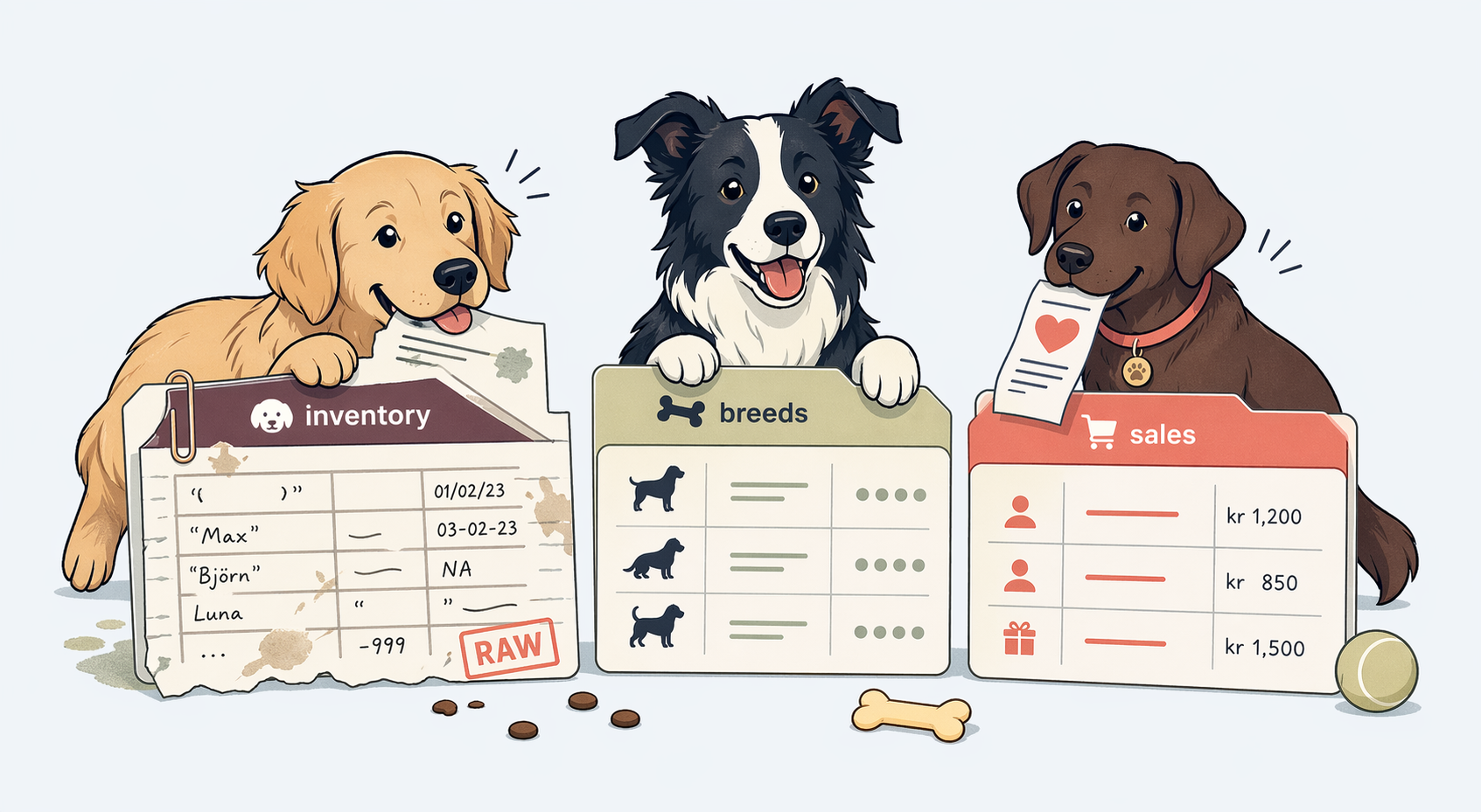
[1] "dog_breeds.csv"    "dog_events.csv"    "dog_inventory.csv" "dog_sales.csv"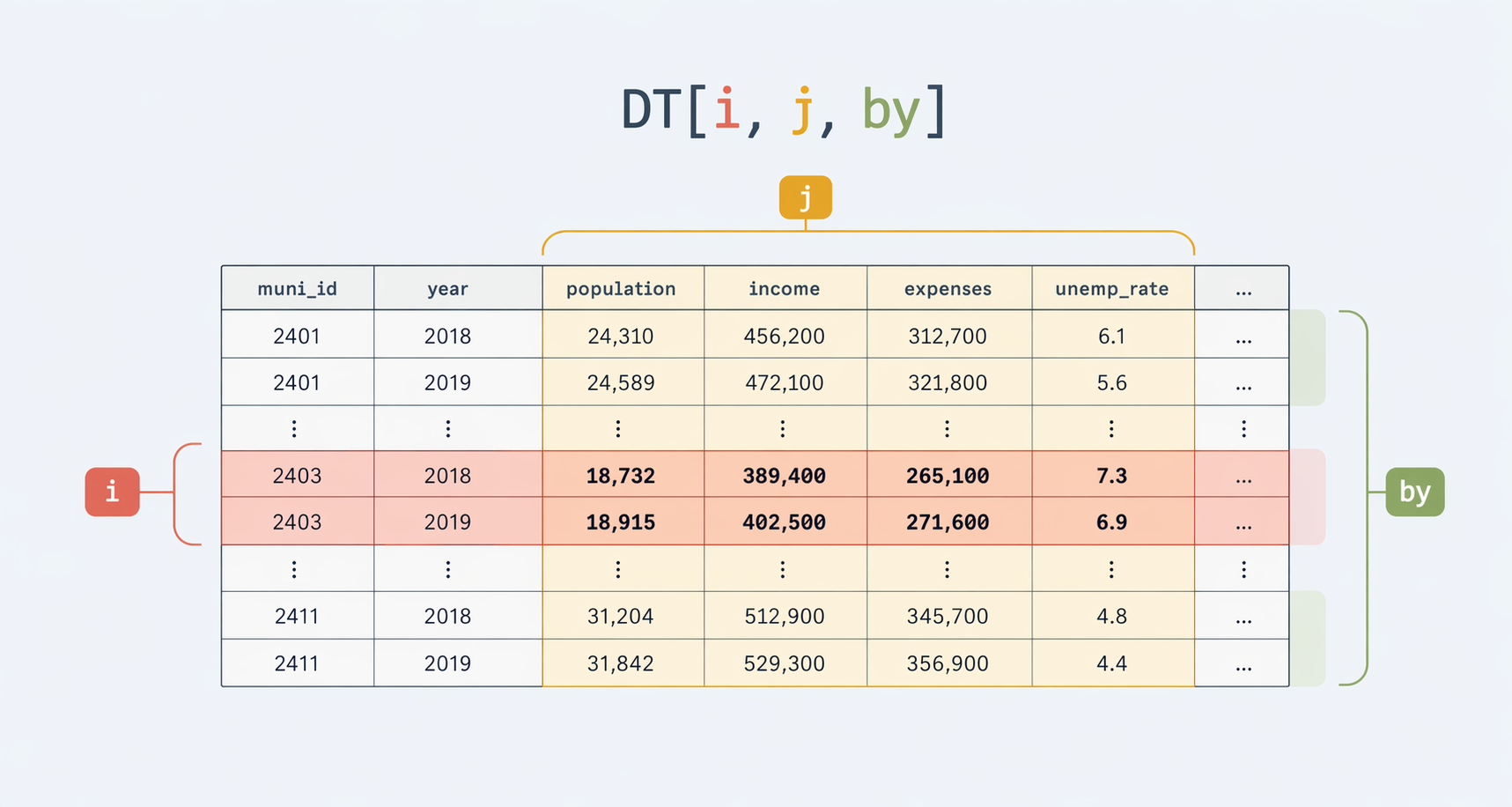    

View your raw data

readLines(dog_path, n = 6)

[1] "Dog Shelter Intake Data - Q1 2025 Records with Pricing and owner Info"           
[2] "Last updated 2025-03-31"                                                         
[3] "---"                                                                             
[4] ""                                                                                
[5] "dog_id,name,breed,age,color,price,insured,intake_date,sale_date,new owner"       
[6] "0013,Buddy,Labrador Retriever,5,Yellow,450.50,1,2023-01-15,03/20-2023,John Smith"

readLines() is just a convenient way to show raw data on a slide; opening the file directly in the IDE works just as well. A messy file often reveals problems before R even parses it: metadata lines above the header, unusual date formats, spaces in variable names, and suspicious codes that probably mean “missing”. Looking at a few raw lines is often faster than guessing from memory.

fread() is forgiving, but can’t solve all issues

fread(dog_path)[3:4]

Warning in fread(dog_path): Discarded single-line footer: <<The data is
computer-generated for educational purposes.>>

   dog_id   name            breed   age  color  price insured intake_date  sale_date
    <int> <char>           <char> <int> <char>  <num>   <int>      <IDat>     <char>
1:   4200    Max Golden Retriever     7 Golden 550.75       0  2023-03-05 06/15-2023
2:   6152  Daisy          Bulldog     4  White 700.00       1  2023-04-20 07/11-2023
         new owner
            <char>
1:   James Johnson
2: Ren\xe9e Dubois

• Good news: fread() found the real header
• Less good: that still does not mean the import is correct

fread() is often great at skipping junk and guessing delimiters. That is helpful, but it can also tempt people into overconfidence. A successful import call is not evidence that the types, encodings, or missing-value rules are correct.

Encoding problems show up in the values

fread(dog_path)[c(4, 6), .(name, `new owner`)]

Warning in fread(dog_path): Discarded single-line footer: <<The data is
computer-generated for educational purposes.>>

      name          new owner
    <char>             <char>
1:   Daisy    Ren\xe9e Dubois
2: L\xfana Sof\xeda M\xfcller

• Computers need to encode characters to store them
• Unfortunately there are tons of different encodings
• A-Z, 0-9 is usually the same, but code for e.g. å can vary
• Can create a real mess…

This is a realistic symptom of encoding trouble: the table loaded, but names with accented characters became broken text. These bugs often go unnoticed until much later, for example during joins, filtering, or plotting.

Tell fread what you know

fread(
  dog_path,
  skip = 3,
  encoding = "Latin-1"
)[c(4, 6), .(name, `new owner`)]

Warning in fread(dog_path, skip = 3, encoding = "Latin-1"): Discarded single-line footer:
<<The data is computer-generated for educational purposes.>>

     name    new owner
   <char>       <char>
1:  Daisy Renée Dubois
2:   Lúna Sofía Müller

• skip = 3 removes the preamble explicitly
• encoding = "Latin-1" tells fread the file is in Latin-1 (an old single-byte Western European encoding)

The general rule is simple: anything known about the file should be encoded in the import call. That is more robust than hoping future guesses will land the same way.

Repairing names

names(fread(dog_path, skip = 3, encoding = "Latin-1"))[9:10]

[1] "sale_date" "new owner"

names(fread(dog_path, skip = 3, encoding = "Latin-1", check.names = TRUE))[9:10]

[1] "sale_date" "new.owner"

check.names = TRUE converts spaces into syntactic names

Name repair is useful when import is messy, but it should be done thoughtfully. The goal is not to let the computer rename things without inspection. The goal is to get names into a form that is easy to reference and unlikely to break code.

To refer to a name with a space we need to enclose it with backticks (``), like in dogs$new owner[5]. Easier to fix at import so we can use dogs$new.owner[5] instead.

Protect identifiers at import time

dogs_bad <- fread(dog_path, skip = 3, encoding = "Latin-1")
dogs_good <- fread(
  dog_path,
  skip = 3,
  encoding = "Latin-1",
  colClasses = list(character = "dog_id")
)

dogs_bad[1:5, dog_id]

[1]   13 3382 4200 6152 8186

dogs_good[1:5, dog_id]

[1] "0013" "3382" "4200" "6152" "8186"

Just like with the municipal data, dog_id is an identifier, not a quantity. If the leading zero disappears, later joins, filters, and duplicate checks will silently become less reliable.

A good import call is explicit

dogs <- fread(
  dog_path,
  skip = 3,
  encoding = "Latin-1",
  check.names = TRUE,
  na.strings = c("", "-99"),
  colClasses = list(character = "dog_id")
)

dogs[1:3, .(dog_id, name, intake_date, sale_date, new.owner)]

   dog_id   name intake_date  sale_date     new.owner
   <char> <char>      <IDat>     <char>        <char>
1:   0013  Buddy  2023-01-15 03/20-2023    John Smith
2:   3382   Lucy  2023-02-10 04/01-2023  Maria Garcia
3:   4200    Max  2023-03-05 06/15-2023 James Johnson

This is not “verbose for the sake of verbosity”. It is a compact contract with the future reader. The ugly details of this file are now visible in one place: skip the preamble, fix the encoding, protect the identifier, repair the names, and treat the fake missing code as missing.

select the columns you use

fread(
  dog_path,
  skip = 3,
  encoding = "Latin-1",
  select = c(
    "dog_id",
    "name",
    "breed",
    "intake_date",
    "sale_date"
  ),
  colClasses = list(character = "dog_id")
)[1:5]

   dog_id    name              breed intake_date  sale_date
   <char>  <char>             <char>      <IDat>     <char>
1:   0013   Buddy Labrador Retriever  2023-01-15 03/20-2023
2:   3382    Lucy    German Shepherd  2023-02-10 04/01-2023
3:   4200     Max   Golden Retriever  2023-03-05 06/15-2023
4:   6152   Daisy            Bulldog  2023-04-20 07/11-2023
5:   8186 Charlie             Beagle  2023-05-11 08/02-2023

Selective import is useful when a file is wide and the first job is just inspection or a focused task. It also reduces noise on slides and in exploratory work. The important thing is to avoid pretending that unused columns are part of the current task.

Importing Stata .dta files with haven

• Use haven::read_dta(). Preserves Stata labels.
• Convert to data.table with as.data.table(),
• Set value labels with as_factors()

library(haven)

stata_dt = read_dta("path/to/stata_file.dta") |>
  as.data.table()

stata_dt[, factor_variable := as_factor(labelled_variable)]

Similarly, we would use haven::write_dta() to save a data frame as a Stata dta file.

Reading excel files with readxl

library(readxl)
excel_dt = read_excel("path/to/spreadsheet.xlsx")

readxl supports selecting sheets:

excel_sheets("path/to/spreadsheet.xlsx")
read_excel("spreadsheet.xlsx", sheet = "Sheet2")

and even specific ranges:

read_excel("spreadsheet.xlsx", range = "A1:D10", skip = 2)

Core data.table Grammar

• Importing Data

• Core data.table Grammar

• Useful data.table Tooling

• Grouping and Summarizing

• Missing Values And Type Repair

• Writing Clean Data

• Using Functions when Wrangling

data.table and dplyr

• Two dominant paradigms for data manipulation in R
• Both are powerful and widely used, but with different syntax
• We will focus on data.table, because it is much faster

data.table: Core concept

• An enhancement of base R’s data.frame
• Fast: Operations implemented in C
• Memory efficient: Modifies by reference using :=
• Indexing: Automatic indexing speeds up subsets and joins
• Concise syntax: Combines operations efficiently

Read DT[i, j, by] as a sentence

“from this table, keep these rows (i), then return (and compute) these columns (j), grouped by these variables (by)”

The small diagram previews the full DT[i, j, by] logic, but the key point on this slide is still the basic i and j split. Once those feel concrete, later grouped work and joins become much easier to understand.

i filters rows

dogs[
  age >= 5 & price > 500,
  .(dog_id, name, breed, age, price)
]

    dog_id     name            breed   age   price
    <char>   <char>           <char> <int>   <num>
 1:   4200      Max Golden Retriever     7  550.75
 2:   4094   Cooper        Dachshund     5  650.50
 3:   6988     Bear            Boxer     6  900.00
---                                               
75:   8279   Bonnie     Irish Setter     7  690.50
76:   9367   Fluffy    Border Collie     8  600.00
77:   0126 Leo King          Whippet     5 1010.50

This is the direct analogue of row filtering: define a logical condition, keep the matching rows, and optionally return only the relevant columns.

i can use membership too

dogs[
  breed %in% c("Pug", "Boxer", "Border Collie") & insured == 1,
  .(dog_id, name, breed, insured)
]

    dog_id   name         breed insured
    <char> <char>        <char>   <int>
 1:   2652   Milo         Boxer       1
 2:   6635  Bella         Boxer       1
 3:   6988   Bear         Boxer       1
---                                    
18:   3599 Brutus           Pug       1
19:   4636  Balto Border Collie       1
20:   2977  Major           Pug       1

%in% is usually clearer than a long chain of | comparisons. It is especially useful for filtering on lists of categories, codes, or allowed values.

%between% filters ranges

dogs[
  price %between% c(400, 700) & age %between% c(2, 5),
  .(dog_id, name, age, price)
]

    dog_id     name   age price
    <char>   <char> <int> <num>
 1:   0013    Buddy     5 450.5
 2:   3382     Lucy     3 600.0
 3:   6152    Daisy     4 700.0
---                            
33:   5497 Clifford     5 680.0
34:   2738   Ripley     2 610.5
35:   5771    Slick     4 670.0

• Shorthand for x >= a & x <= b, both endpoints included
• Reads closer to intent than a chained comparison

A small piece of syntax, but range filters appear constantly in wrangling. The inclusive-on-both-ends behaviour matches the usual reading of “between 400 and 700”.

j selects columns

dogs[
  ,
  .(dog_id, name, breed, age, price, insured)
]

     dog_id     name              breed   age   price insured
     <char>   <char>             <char> <int>   <num>   <int>
  1:   0013    Buddy Labrador Retriever     5  450.50       1
  2:   3382     Lucy    German Shepherd     3  600.00       1
  3:   4200      Max   Golden Retriever     7  550.75       0
 ---                                                         
169:   8857    Snowy              Corgi     2  990.00      NA
170:   0126 Leo King            Whippet     5 1010.50       0
171:   8159      Tut            Whippet     0  750.75       1

The .() notation is just a convenient shorthand for list(). In data.table, that list of columns becomes a table again.

j can compute new outputs

dogs[
  age > 0,
  .(
    dog_id,
    name,
    breed,
    price_per_year = round(price / age, 1)
  )
][1:8]

   dog_id    name              breed price_per_year
   <char>  <char>             <char>          <num>
1:   0013   Buddy Labrador Retriever           90.1
2:   3382    Lucy    German Shepherd          200.0
3:   4200     Max   Golden Retriever           78.7
4:   6152   Daisy            Bulldog          175.0
5:   8186 Charlie             Beagle           50.0
6:   1893    Lúna            Bulldog          400.0
7:   4094  Cooper          Dachshund          130.1
8:   1099   Sadie          Dachshund           50.0

This is a good example of why j is more than “select columns”. It is the place where new columns or summaries are created from existing ones.

:= modifies by reference

dogs_work <- copy(dogs)

dogs_work[, price_per_year := fifelse(
  age > 0,
  round(price / age, 1),
  NA_real_
)]

dogs_work[
  1:5,
  .(dog_id, name, age, price, price_per_year)
]

   dog_id    name   age  price price_per_year
   <char>  <char> <int>  <num>          <num>
1:   0013   Buddy     5 450.50           90.1
2:   3382    Lucy     3 600.00          200.0
3:   4200     Max     7 550.75           78.7
4:   6152   Daisy     4 700.00          175.0
5:   8186 Charlie     6 300.25           50.0

This is one of the most important data.table differences from copy-heavy workflows. := changes the existing object in memory. That is powerful and efficient, but it requires deliberate handling whenever a separate copy is needed. If one new column depends on another, the safe pattern is two steps or a chained operation, not a single := call that quietly relies on evaluation order.

Use copy() when you need separation

"price_per_year" %in% names(dogs)

[1] FALSE

"price_per_year" %in% names(dogs_work)

[1] TRUE

This small check makes the point visible. We created dogs_work from copy(dogs), so the new column appears only in the copy. Without copy(), the original object would also have been changed.

Comparison to dplyr

• Part of the Tidyverse collection of packages
• Focuses on readability and consistency
• Uses distinct “verbs” for common operations

data.table

data[condition,
     .(new_var = mean(old_var)),
     by = "group_var"]

dplyr

data |>
  filter(condition) |>
  group_by(group_var) |>
  summarise(new_var = mean(old_var))

If you really like the dplyr syntax but want to take advantage of data.table speeds, there is the dtplyr package which uses data.table as a backend for dplyr-syntax operations.

data.table vs. dplyr - key differences

data.table

• Pros: Speed, memory efficiency, concise syntax, powerful indexing/joins. Ideal for large data.
• Cons: Steeper learning curve, syntax less “English-like”, modify-by-reference needs care.

dplyr

• Pros: Highly readable verbs, Tidyverse integration (ggplot2, etc.).
• Cons: Slower, uses more memory, especially on large data or complex groups.

Useful data.table Tooling

• Importing Data

• Core data.table Grammar

• Useful data.table Tooling

• Grouping and Summarizing

• Missing Values And Type Repair

• Writing Clean Data

• Using Functions when Wrangling

Setting a key creates an index for faster operations

dogs[, .(dog_id, name, breed)][1:2]

   dog_id   name              breed
   <char> <char>             <char>
1:   0013  Buddy Labrador Retriever
2:   3382   Lucy    German Shepherd

setkey(dogs, dog_id, breed)
dogs[, .(dog_id, name, breed)][1:2]

Key: <dog_id, breed>
   dog_id   name              breed
   <char> <char>             <char>
1:   0009  Scout      Border Collie
2:   0013  Buddy Labrador Retriever

setkey() does two things at once: it sorts the table by the chosen columns and stores them as the key. The visible change above is just the sort. The invisible change is that subsequent subsets and joins on those columns now use binary search instead of a linear scan, which matters for large tables.

setkey() automatically sorts the data table by the key.

Removing columns by reference with := NULL

dogs_work[, price_per_year := NULL]
"price_per_year" %in% names(dogs_work)

[1] FALSE

Because := changes the table by reference, deletion is also explicit. This is useful when a temporary helper column did its job and should not leak into later analysis.

Renaming and reordering by reference

dogs_demo <- copy(dogs)

setnames(dogs_demo, c("new.owner", "intake_date"), c("owner", "intake"))
setcolorder(dogs_demo, c("dog_id", "name", "breed", "owner"))

names(dogs_demo)

 [1] "dog_id"    "name"      "breed"     "owner"     "age"       "color"     "price"    
 [8] "insured"   "intake"    "sale_date"

• := NULL deletes
• setnames() renames
• setcolorder() reorders

Like :=, both functions change the table in place without making a copy. That makes them fast on large tables, but the same caveat applies: they mutate the object passed in. Use copy() first when separation matters.

fcase() is cleaner than nested ifelse()

dogs_work[, fee_group := fcase(
  price < 400, "low",
  price < 700, "middle",
  default = "high"
)]

dogs_work[, .(dog_id, name, price, fee_group)]

     dog_id     name   price fee_group
     <char>   <char>   <num>    <char>
  1:   0013    Buddy  450.50    middle
  2:   3382     Lucy  600.00    middle
  3:   4200      Max  550.75    middle
 ---                                  
169:   8857    Snowy  990.00      high
170:   0126 Leo King 1010.50      high
171:   8159      Tut  750.75      high

This is one of the practical data.table conveniences worth teaching early. Nested ifelse() calls become unreadable quickly. fcase() makes mutually exclusive categories much easier to inspect.

Diagnose distinct values and duplicates

dogs[, .(
  rows = .N,
  distinct_ids = uniqueN(dog_id),
  distinct_breeds = uniqueN(breed)
)]

    rows distinct_ids distinct_breeds
   <int>        <int>           <int>
1:   171          170              21

dogs[duplicated(dogs, by = "dog_id"), .(dog_id, name)]

   dog_id   name
   <char> <char>
1:   4200    Max

dim(unique(dogs, by = "dog_id"))

[1] 170  10

• uniqueN() counts distinct values; unique() returns them
• uniqueN(key) == nrow(dt) is a one-line uniqueness test
• duplicated(dt, by = ...) lists offending rows
• unique(dt, by = ...) keeps one row per key

A duplicated identifier is a quiet bug. It will not stop the script, but it will silently inflate joins and break aggregations. Pairing .N with uniqueN() is one of the most useful first-look diagnostics after import, and unique(dt, by = key) is the matching fix when duplicates appear. This sets up the join-key checks that lecture 7 leans on.

Piping with data.table

• data.table supports the native pipe |>
• Use _ as a placeholder for the output of the previous step

dogs |>
  _[age > 0] |>
  _[, price_per_yr := round(price / age)] |>
  _[order(-price_per_yr)] |>
  _[, .(dog_id, name, price_per_yr)]

     dog_id     name price_per_yr
     <char>   <char>        <num>
  1:   6447 Hercules         1000
  2:   6941   Zephyr          950
  3:   9866   Cherry          790
 ---                             
160:   6197    Benji           49
161:   6596    Oscar           46
162:   1976    Honey           41

The first _[age > 0] returns a new filtered table, so the later := modifies that table, not dogs. Skipping the filter step (dogs |> _[, := ...]) would have written the new column straight into dogs. Mixing := into a pipe is fine, but the upstream step has to actually produce a copy.

Grouping and Summarizing

• Importing Data

• Core data.table Grammar

• Useful data.table Tooling

• Grouping and Summarizing

• Missing Values And Type Repair

• Writing Clean Data

• Using Functions when Wrangling

Grouping and summarizing with by=

• i chooses rows
• j says what to return or compute
• by says which groups should get separate answers

Grouping and summarizing with by= (cont.)

Evaluate j separately for each group:

dogs[, mean(price), by = .(insured)]

   insured       V1
     <int>    <num>
1:       0 651.2295
2:       1 735.3387
3:      NA 810.1875

Can group by multiple variables, and by conditions:

dogs[, mean(price), 
     by = .(insured, 
            white = color == "White")]

   insured  white       V1
     <int> <lgcl>    <num>
1:       0  FALSE 651.4461
2:       1  FALSE 735.5226
3:       1   TRUE 733.7500
4:       0   TRUE 650.1250
5:      NA  FALSE 883.3333
6:      NA   TRUE 590.7500

Grouping and summarizing with by= (cont.)

Find cheapest dog by breed, ordered by how frequent the breed is

dogs[, .(.N, min(price)), by = "breed"] |>
  _[order(-N)]

                       breed     N     V2
                      <char> <int>  <num>
 1:                      Pug    16 600.00
 2:                  Whippet    15 560.00
 3:            Border Collie    13 510.00
---                                      
19:          Irish Wolfhound     4 840.25
20:                  Bulldog     3 700.00
21: Chesapeake Bay Retriever     2 720.00

Grouped counts are useful diagnostics

dogs[, .(
  rows = .N,
  missing_sale_date = sum(is.na(sale_date)),
  insured_share = round(mean(insured == 1, na.rm = TRUE), 2)
), by = breed][order(-rows)]

                       breed  rows missing_sale_date insured_share
                      <char> <int>             <int>         <num>
 1:                      Pug    16                 3          0.73
 2:                  Whippet    15                 4          0.71
 3:            Border Collie    13                 2          0.31
---                                                               
19:          Irish Wolfhound     4                 2          1.00
20:                  Bulldog     3                 1          1.00
21: Chesapeake Bay Retriever     2                 0          1.00

Grouped summaries are not just for presentation. They are also diagnostic tools. A quick count by category can reveal sparse groups, missing values concentrated in one group, or unexpected coding patterns.

Transforming with := and by=

Saving the average price by age to a new column, repeating the summary for each row in group:

dogs[, avg_price_by_age := mean(price),
     by = .(age)]

dogs[order(age),
     .(age, avg_price_by_age)]

       age avg_price_by_age
     <int>            <num>
  1:    -5        1120.0000
  2:    -4         820.0000
  3:    -3         740.5000
 ---                       
169:    10         545.3125
170:    10         545.3125
171:    11         540.0000

Grouped transformations create new columns

copy(dogs) |>
  _[, price_gap_from_breed_mean :=
    price - mean(price, na.rm = TRUE),
    by = breed] |>
  _[breed %in% c("Pug", "Boxer"),
    .(dog_id, name, breed, price, price_gap_from_breed_mean)]

Key: <dog_id, breed>
    dog_id     name  breed  price price_gap_from_breed_mean
    <char>   <char> <char>  <num>                     <num>
 1:   1927   Oliver    Pug 750.00                 -95.82812
 2:   2370     Juno    Pug 910.00                  64.17188
 3:   2646 Snowball    Pug 620.50                -225.32812
---                                                        
21:   8522    Rocky  Boxer 500.00                -177.30714
22:   9883    Simba    Pug 930.00                  84.17188
23:   9988    Ziggy  Boxer 610.25                 -67.05714

The grouped mean is repeated within each group because this is a grouped transformation, not a grouped collapse. That distinction matters. Summaries reduce rows; transformations keep the original rows.

.SD

Inside a data.table, .SD refers to the Subset of Data for each group.

We can use this to run more complex operations, like

dogs[, lapply(.SD, func), by = ...]

applying a custom function func to each .SD group.

.SD is also a data.table

.SDcols

Specifies the columns included in .SD. Can be used to select columns in smart ways.

dogs[, c(
  list(dogs = .N),
  lapply(.SD, function(x) round(mean(x, na.rm = TRUE), 2))
), by = breed, .SDcols = c("age", "price")]

                 breed  dogs   age  price
                <char> <int> <num>  <num>
 1:      Border Collie    13  5.00 678.60
 2: Labrador Retriever     6  3.00 708.71
 3:            Whippet    15  3.87 739.70
---                                      
19:          Dalmatian    12  5.00 658.62
20:       Irish Setter    10  4.90 676.28
21:             Beagle     7  5.14 536.00

Use shift() to create a lagged vector

shift() returns a lagged vector within groups

events

    dog_id          event_time event_type           shelter_name staff_id event_date
    <char>              <POSc>     <char>                 <char>   <char>     <IDat>
 1:   0013 2023-01-15 08:42:00     intake     Happy Paws Shelter      A12 2023-01-15
 2:   0013 2023-03-20 23:40:00    adopted     Happy Paws Shelter      B07 2023-03-20
 3:   3382 2023-02-10 09:05:00     intake       City Animal Care      A12 2023-02-10
---                                                                                 
81:   1254 2023-09-16 13:25:00  vet_check     Happy Paws Shelter      V01 2023-09-16
82:   4094 2023-09-04 14:50:00  vet_check     Happy Paws Shelter      V01 2023-09-04
83:   5522 2024-01-08 10:20:00  vet_check Willow Creek Adoptions      V03 2024-01-08

setorder(events, dog_id, event_time) # setorder() is crucial!
events[,
  hours_since_previous_event := round(
    as.numeric(difftime(event_time, shift(event_time), units = "hours")), 1
  ),
  by = dog_id
]
events[
  dog_id %in% c("0013", "3382"),
  .(dog_id, event_time, event_type, hours_since_previous_event)
]

   dog_id          event_time event_type hours_since_previous_event
   <char>              <POSc>     <char>                      <num>
1:   0013 2023-01-15 08:42:00     intake                         NA
2:   0013 2023-03-20 23:40:00    adopted                     1551.0
3:   3382 2023-02-10 09:05:00     intake                         NA
4:   3382 2023-02-13 14:30:00  vet_check                       77.4
5:   3382 2023-04-01 11:30:00    adopted                     1124.0

Missing Values And Type Repair

• Importing Data

• Core data.table Grammar

• Useful data.table Tooling

• Grouping and Summarizing

• Missing Values And Type Repair

• Writing Clean Data

• Using Functions when Wrangling

Missing values are a workflow issue

• Some missings are genuine unknowns
• Some are fake codes like -99
• Some are actually impossible values that should become NA

It is useful to separate three ideas: a value that is truly unavailable, a code that means unavailable, and a recorded value that is simply wrong. They should not all be treated the same way.

Code fake missings at read time when you can

dogs_raw <- fread(dog_path, skip = 3, encoding = "Latin-1")
dogs <- fread(
  dog_path,
  skip = 3,
  encoding = "Latin-1",
  check.names = TRUE,
  na.strings = c("", "-99"),
  colClasses = list(character = "dog_id")
)

unique(dogs_raw$insured)

[1]   1   0  NA -99

unique(dogs$insured)

[1]  1  0 NA

This is a clean example of a rule that should live in the import step. If -99 means missing, it is better to say so once while reading the file than to remember that fact in three later scripts.

Use is.na() explicitly

dogs[is.na(insured), .(dog_id, name, insured)]

   dog_id    name insured
   <char>  <char>   <int>
1:   6015 Patches      NA
2:   6941  Zephyr      NA
3:   4890  Anubis      NA
4:   8857   Snowy      NA

Comparisons like x == NA do not work the way beginners expect. Missingness should be checked with is.na() so the intention is explicit and correct.

Some values are not missing, just wrong

dogs[age < 0, .(dog_id, name, age)]

   dog_id    name   age
   <char>  <char> <int>
1:   6455    Coco    -1
2:   6859  Härley    -3
3:   4967    Növa    -2
4:   6301 Düke II    -4
5:   5131     Rex    -2
6:   7690  Wolfie    -5

Negative ages are not a plausible substantive value here. They should not stay in the data as if they were meaningful. This is a good example of an “impossible value” rather than a pre-coded missing.

Repair obvious problems explicitly

dogs_fixed <- copy(dogs)
dogs_fixed[age < 0, age := NA_integer_]

dogs_fixed[, .(
  missing_age = sum(is.na(age)),
  missing_sale_date = sum(is.na(sale_date)),
  missing_insured = sum(is.na(insured))
)]

   missing_age missing_sale_date missing_insured
         <int>             <int>           <int>
1:           6                37               4

The pattern matters more than this specific example: identify the impossible condition, change only the affected rows, and then verify the result with a small count.

fcoalesce() fills missings with a default

dogs_fixed[, owner_label := fcoalesce(new.owner, "not yet sold")]

dogs_fixed[
  is.na(new.owner),
  .(dog_id, name, new.owner, owner_label)
][1:5]

   dog_id    name new.owner  owner_label
   <char>  <char>    <char>       <char>
1:   6988    Bear      <NA> not yet sold
2:   8380    Ruby      <NA> not yet sold
3:   8774    Duke      <NA> not yet sold
4:   1288   Penny      <NA> not yet sold
5:   8853 Winston      <NA> not yet sold

• Returns the first non-NA value, argument by argument
• Replaces nested ifelse(is.na(x), y, x) patterns
• Accepts more than two arguments: fcoalesce(a, b, c)

fcoalesce() is the SQL COALESCE idea. The multi-argument form is useful when several columns hold the same logical value and the goal is the first that is actually populated, for example fcoalesce(reported_date, recorded_date, intake_date).

Date parsing is a type problem too

class(dogs$intake_date)

[1] "IDate" "Date" 

class(dogs$sale_date)

[1] "character"

• intake_date was parsed as IDate (data.table’s date type, inherits from Date)
• sale_date is still text — the 03/20-2023 format wasn’t recognized

This is intentionally a bridge to lecture 7. Date handling is not a separate universe; it is a special case of getting types right. If a date is still a character string, date arithmetic will not work reliably.

Parse the dates explicitly

dogs_fixed[, sale_date := as.IDate(sale_date, format = "%m/%d-%Y")]

class(dogs_fixed$sale_date)

[1] "IDate" "Date" 

dogs_fixed[1:3, .(dog_id, intake_date, sale_date)]

   dog_id intake_date  sale_date
   <char>      <IDat>     <IDat>
1:   0013  2023-01-15 2023-03-20
2:   3382  2023-02-10 2023-04-01
3:   4200  2023-03-05 2023-06-15

• as.IDate() parses text into IDate, given the format string
• %m/%d-%Y matches 03/20-2023: month, /, day, -, four-digit year

Format strings come from strptime(). Common pieces: %Y four-digit year, %y two-digit year, %m month, %d day. Lecture 7 covers the rest.

Writing Clean Data

• Importing Data

• Core data.table Grammar

• Useful data.table Tooling

• Grouping and Summarizing

• Missing Values And Type Repair

• Writing Clean Data

• Using Functions when Wrangling

Separate raw, processed, and analysis steps

• Raw files are inputs
• Processed files are reproducible intermediate outputs
• Analysis starts from processed data, not from manual edits

This mirrors the project-workflow lecture. A processed file is useful when the cleaning work is non-trivial and should not be repeated interactively from memory. It also creates a clear surface for version control and debugging.

Write a cleaned file with fwrite()

out_dir <- file.path(tempdir(), "ec7422-wrangling")
dir.create(out_dir, showWarnings = FALSE)

out_path <- file.path(out_dir, "dogs_clean.csv")
fwrite(dogs_fixed, out_path)

Read it back and verify

dogs_roundtrip <- fread(
  out_path,
  colClasses = list(character = "dog_id")
)
dogs_roundtrip[1:3, .(dog_id, name, age, sale_date)]

   dog_id   name   age  sale_date
   <char> <char> <int>     <IDat>
1:   0013  Buddy     5 2023-03-20
2:   3382   Lucy     3 2023-04-01
3:   4200    Max     7 2023-06-15

Note how we still need be explicit about some types when re-importing. The information is not stored in the CSV.

Using Functions when Wrangling

• Importing Data

• Core data.table Grammar

• Useful data.table Tooling

• Grouping and Summarizing

• Missing Values And Type Repair

• Writing Clean Data

• Using Functions when Wrangling

Repetition is the best reason to write a function

• repeated import rules
• repeated validation checks
• repeated cleaning with one file path changed
• repeated summaries that should agree exactly

This is the practical reason to care about functions in a wrangling workflow. The gain is not elegance for its own sake. The gain is one stable place for logic that would otherwise get copied, edited, and slowly broken.

A wrangling function should show its contract

• explicit arguments
• one clear output
• no hidden dependence on objects in the global environment
• one place to store the weird file-specific rules

This is the level of functions that matters most in applied data work. A small explicit function is easier to inspect than a long script with near-duplicate code blocks scattered through it.

Put the dog import rules in one place

read_dogs <- function(path) {
  fread(
    path,
    skip = 3,
    encoding = "Latin-1",
    check.names = TRUE,
    na.strings = c("", "-99"),
    colClasses = list(character = "dog_id")
  )
}

read_dogs(dog_path)[
  1:3,
  .(dog_id, name, intake_date, sale_date)
]

   dog_id   name intake_date  sale_date
   <char> <char>      <IDat>     <char>
1:   0013  Buddy  2023-01-15 03/20-2023
2:   3382   Lucy  2023-02-10 04/01-2023
3:   4200    Max  2023-03-05 06/15-2023

This is already useful even before any advanced programming ideas show up. The messy import rules now live in one place, and future code can call the function without retyping them.

Hidden globals make even simple functions misleading

bad_oldest <- function(dt) dogs[which.max(age), .(dog_id, name, age)]
oldest_dog <- function(dt) dt[which.max(age), .(dog_id, name, age)]

puppies <- dogs[age <= 2]

bad_oldest(puppies)

   dog_id   name   age
   <char> <char> <int>
1:   6197  Benji    11

oldest_dog(puppies)

   dog_id   name   age
   <char> <char> <int>
1:   1893   Lúna     2

The two signatures look identical, but the behavior is not. bad_oldest declares an argument dt and silently ignores it, falling back to the global dogs — so bad_oldest(puppies) returns the oldest dog overall, not the oldest puppy. oldest_dog actually uses dt. Hidden global lookups are easy to miss in code review and only surface once the global object is renamed, mutated, or no longer in scope.

Returning a table keeps the effect visible

add_senior_flag <- function(dt, age_cutoff = 7L) {
  out <- copy(dt)
  out[, senior := age >= age_cutoff]
  out
}

add_senior_flag(dogs)[, .(dog_id, age, senior)]

     dog_id   age senior
     <char> <int> <lgcl>
  1:   0013     5  FALSE
  2:   3382     3  FALSE
  3:   4200     7   TRUE
 ---                    
169:   8857     2  FALSE
170:   0126     5  FALSE
171:   8159     0  FALSE

When using data.tables as arguments we need to take extra care with the editing copy-vs-reference issue. If we want the function to return a modified table without changing the original, we need to make a copy inside the function and return that copy.

Default arguments keep small helpers flexible

add_senior_flag(dogs)[, .N, by = senior]

   senior     N
   <lgcl> <int>
1:  FALSE   131
2:   TRUE    40

add_senior_flag(dogs, age_cutoff = 9L)[, .N, by = senior]

   senior     N
   <lgcl> <int>
1:  FALSE   159
2:   TRUE    12

Default arguments are useful when one rule is common but not universal. Most calls can use the default, while the rare special case can still be handled without copying the function body and editing it by hand.

Main takeaways

• A successful import is not the same as a correct import
• Inspect names, types, keys, and missingness immediately
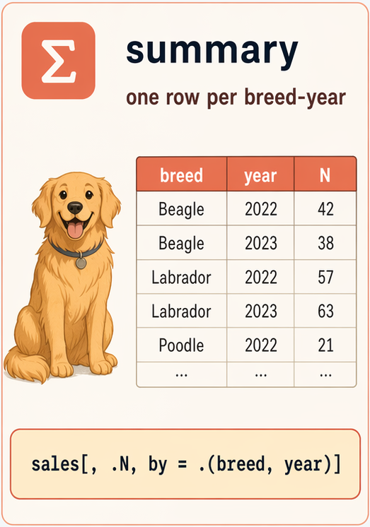
• Read DT[i, j, by] as “i=rows, j=columns/calculations, by=groups”
• Use := deliberately and copy() when you need separation

Next lecture: advanced wrangling