Lecture 4: R Basics II: Vectors, Tables, and Tidy Thinking

EC7422: Data Science for Economic Analysis

Adam Altmejd Selder

adam.altmejd@su.se

The Institute for Evaluation of Labour Market and Education Policy (IFAU)

April 16, 2026

Today

From single values to vectors
From vectors to tables
Table access and column work
Keys, factors, tidy data
Checks and quick plots

Review: lecture 3 in one minute

Expressions evaluate to values
Assignment binds names to objects
Types affect behavior
Logic and if / else control decisions
Functions package reusable work

Vectors

Vectors
From Vectors To Tables
Subsetting Tables
Working With Table Columns
Categories
Tidy Data
Basic Checks
Quick Inspection Plots

A vector stores many values of one type

scores <- c(45, 62, 78)
scores

[1] 45 62 78

One name for many values
Values stay in order
One object in memory

Mixed values are coerced

If you try to mix values, R will force them to a common type:

survey_answers <- c(1, 2, "3")
survey_answers

[1] "1" "2" "3"

typeof(survey_answers)

[1] "character"

One vector, one type
Coercion can be silent and cause bugs

Logical operators evaluate each pair of elements

scores >= 60

[1] FALSE  TRUE  TRUE

scores >= 60 & scores < 75

[1] FALSE  TRUE FALSE

Same operators as before
One result per element: a logical vector

typeof(scores >= 60)

[1] "logical"

Be wary of recycling

c(1, 2, 3) > c(1, 3)

Warning in c(1, 2, 3) > c(1, 3): longer object length is not a
multiple of shorter object length

[1] FALSE FALSE  TRUE

Shorter vector may repeat
Sometimes warning
Sometimes silent

“Vectorized” functions operate element by element

trial <- c(1, NA, 3)
is.na(trial)

[1] FALSE  TRUE FALSE

!is.na(trial)

[1]  TRUE FALSE  TRUE

Same is.na()
One result per element
Useful before filtering

Use `%in%` to check membership

cities <- c("stockholm", "uppsala", "umea")
cities %in% c("stockholm", "malmo", "uppsala")

[1]  TRUE  TRUE FALSE

Membership in a reference set
One result per element

Often clearer than many |:

cities == "stockholm" | cities == "malmo" | cities == "uppsala"

[1]  TRUE  TRUE FALSE

`ifelse()` builds a new vector

The if / else pattern requires condition to be a single logical value. If you want to apply the same logic to many values, ifelse() is the vectorized alternative:

ifelse(scores >= 60, "pass", "retry")

[1] "retry" "pass"  "pass"

Condition checked element by element
Output has matching length
Useful for quick categories

Subset by position with `[]`

years <- c(2021, 2022, 2023, 2024)
years[1]

[1] 2021

Position-based subsetting
One element or several
Fundamental operator in R

Use : to create a sequence of integers:

2:4

[1] 2 3 4

years[2:4]

[1] 2022 2023 2024

Subset by logical vector with `[]`

Use a same-length logical vector to keep matching elements:

years[c(TRUE, FALSE, TRUE, FALSE)]

[1] 2021 2023

Subset by condition with `[]`

Or let a condition evaluate to a logical vector on the fly:

scores[scores >= 60]

[1] 62 78

years[years >= 2023]

[1] 2023 2024

This is what we use to filter table rows!

Vectors can replace loops

out <- numeric(length(scores))
for (i in seq_along(scores)) {
  out[i] <- scores[i]^2
}
out

[1] 2025 3844 6084

scores^2

[1] 2025 3844 6084

Same result
Loop is explicit
Vector form is shorter and often faster

A list can hold different kinds of objects

student_record <- list(name = "Alice", age = 24, passed = TRUE)
student_record

$name
[1] "Alice"

$age
[1] 24

$passed
[1] TRUE

typeof(student_record)

[1] "list"

Flexible container
Mixed object types allowed

From Vectors To Tables

Vectors
From Vectors To Tables
Subsetting Tables
Working With Table Columns
Categories
Tidy Data
Basic Checks
Quick Inspection Plots

Start with three column vectors

A table is really just a collection of equal-length vectors. Let’s build one:

municipality_code <- c("0180", "1280")
year <- c(2023, 2023)
unemployment_rate <- c(6.2, 7.1)

Collect them in a list

table_list <- list(
  municipality_code,
  year,
  unemployment_rate
)
table_list

[[1]]
[1] "0180" "1280"

[[2]]
[1] 2023 2023

[[3]]
[1] 6.2 7.1

Give the columns names

table_list <- list(
  municipality_code = municipality_code,
  year = year,
  unemployment_rate = unemployment_rate
)
table_list

$municipality_code
[1] "0180" "1280"

$year
[1] 2023 2023

$unemployment_rate
[1] 6.2 7.1

Data frames

data.frame() is the built-in way of doing this

table_df <- data.frame(
  municipality_code,
  year,
  unemployment_rate
)
table_df

  municipality_code year unemployment_rate
1              0180 2023               6.2
2              1280 2023               7.1

Note how the naming is implicit.

Under the hood

data.frame is just a named equal-length list:

typeof(table_df)

[1] "list"

str(table_df)

'data.frame':   2 obs. of  3 variables:
 $ municipality_code: chr  "0180" "1280"
 $ year             : num  2023 2023
 $ unemployment_rate: num  6.2 7.1

str(table_list)

List of 3
 $ municipality_code: chr [1:2] "0180" "1280"
 $ year             : num [1:2] 2023 2023
 $ unemployment_rate: num [1:2] 6.2 7.1

A matrix is something else

Matrices are also rectangular, but they hold one common type:

as.matrix(table_df)

     municipality_code year   unemployment_rate
[1,] "0180"            "2023" "6.2"            
[2,] "1280"            "2023" "7.1"

typeof(as.matrix(table_df))

[1] "character"

Still rows and columns, but stored as a single vector
One common type for all cells

The municipal panel from Lecture 1

panel_df <- read.csv("../lecture_1/lecture_1_demo_panel.csv")
head(panel_df)

  municipality_code municipality_name year unemployment_rate
1               114    Upplands Väsby 2016              11.9
2               115        Vallentuna 2016               6.1
3               117         Österåker 2016               7.2
4               120            Värmdö 2016               7.3
5               123          Järfälla 2016              13.7
6               125             Ekerö 2016               5.6

Inspect before doing anything else

str(panel_df)

'data.frame':   2320 obs. of  4 variables:
 $ municipality_code: int  114 115 117 120 123 125 126 127 128 136 ...
 $ municipality_name: chr  "Upplands Väsby" "Vallentuna" "Österåker" "Värmdö" ...
 $ year             : int  2016 2016 2016 2016 2016 2016 2016 2016 2016 2016 ...
 $ unemployment_rate: num  11.9 6.1 7.2 7.3 13.7 5.6 12 17.7 9.7 11.9 ...

Also try View(panel_df) in VsCode for an interactive viewer.

Ask five questions first

What is one observation/row?
What is the key?
Which columns:
- identify?
- measure?
- label?

Count rows and columns

nrow(panel_df)

[1] 2320

ncol(panel_df)

[1] 4

Check the variable names

names(panel_df)

[1] "municipality_code" "municipality_name" "year"             
[4] "unemployment_rate"

What is the key?

A database concept: the key is a set of columns that uniquely identifies one observation

municipality_code + year
Not municipality name, that is a label

Identifier versus label

Code = identifier
Name = label
Identifier for matching
Label for humans

Leading zeroes matter

str(panel_df)

'data.frame':   2320 obs. of  4 variables:
 $ municipality_code: int  114 115 117 120 123 125 126 127 128 136 ...
 $ municipality_name: chr  "Upplands Väsby" "Vallentuna" "Österåker" "Värmdö" ...
 $ year             : int  2016 2016 2016 2016 2016 2016 2016 2016 2016 2016 ...
 $ unemployment_rate: num  11.9 6.1 7.2 7.3 13.7 5.6 12 17.7 9.7 11.9 ...

panel_df <- read.csv(
  "../lecture_1/lecture_1_demo_panel.csv",
  colClasses = c(municipality_code = "character")
)
str(panel_df)

'data.frame':   2320 obs. of  4 variables:
 $ municipality_code: chr  "0114" "0115" "0117" "0120" ...
 $ municipality_name: chr  "Upplands Väsby" "Vallentuna" "Österåker" "Värmdö" ...
 $ year             : int  2016 2016 2016 2016 2016 2016 2016 2016 2016 2016 ...
 $ unemployment_rate: num  11.9 6.1 7.2 7.3 13.7 5.6 12 17.7 9.7 11.9 ...

Subsetting Tables

Vectors
From Vectors To Tables
Subsetting Tables
Working With Table Columns
Categories
Tidy Data
Basic Checks
Quick Inspection Plots

A table column is just a vector

$ pulls the column out, then [] subsets that vector like before

panel_df$year[1]

[1] 2016

panel_df$year[1:5]

[1] 2016 2016 2016 2016 2016

On data.frame: `[]` keeps table, `[[]]`, `$` pulls vector

[] returns a one-column table

head(panel_df["year"])

[[]] returns the vector inside

head(panel_df[["year"]])

[1] 2016 2016 2016 2016 2016 2016

Subsetting both rows and columns with `[]`

panel_df[1:3, c("municipality_name", "year")]

  municipality_name year
1    Upplands Väsby 2016
2        Vallentuna 2016
3         Österåker 2016

First slot = rows
Second slot = columns

Filter with logic

Works just like vector filtering, but keeps the table shape:

panel_df[
  panel_df$year == 2023 &
  panel_df$municipality_name %in% c("Stockholm", "Uppsala", "Kiruna"),
  c("municipality_name", "year", "unemployment_rate")
]

     municipality_name year unemployment_rate
2047         Stockholm 2023              10.5
2062           Uppsala 2023               9.9
2320            Kiruna 2023               5.3

Filtering keeps row meaning

panel_df[
  panel_df$municipality_code %in% c("0180", "0380", "1280") &
  panel_df$year %in% c(2022, 2023),
]

     municipality_code municipality_name year unemployment_rate
1757              0180         Stockholm 2022              10.5
1772              0380           Uppsala 2022              10.2
1857              1280             Malmö 2022              18.0
2047              0180         Stockholm 2023              10.5
2062              0380           Uppsala 2023               9.9
2147              1280             Malmö 2023              17.7

Fewer rows
Same observation
Note , at the end to keep all columns

Working With Table Columns

Vectors
From Vectors To Tables
Subsetting Tables
Working With Table Columns
Categories
Tidy Data
Basic Checks
Quick Inspection Plots

Assigning to a new column

We can create a new column by assigning to a name that doesn’t exist yet:

panel_df$high_unemployment <- panel_df$unemployment_rate > 8
head(panel_df[c("municipality_name", "unemployment_rate", "high_unemployment")])

  municipality_name unemployment_rate high_unemployment
1    Upplands Väsby              11.9              TRUE
2        Vallentuna               6.1             FALSE
3         Österåker               7.2             FALSE
4            Värmdö               7.3             FALSE
5          Järfälla              13.7              TRUE
6             Ekerö               5.6             FALSE

`ifelse()` can build categories

panel_df$period <- ifelse(panel_df$year >= 2020, "recent", "older")
head(panel_df[c("year", "period")])

  year period
1 2016  older
2 2016  older
3 2016  older
4 2016  older
5 2016  older
6 2016  older

Tidy Data

Vectors
From Vectors To Tables
Subsetting Tables
Working With Table Columns
Categories
Tidy Data
Basic Checks
Quick Inspection Plots

Tidy data

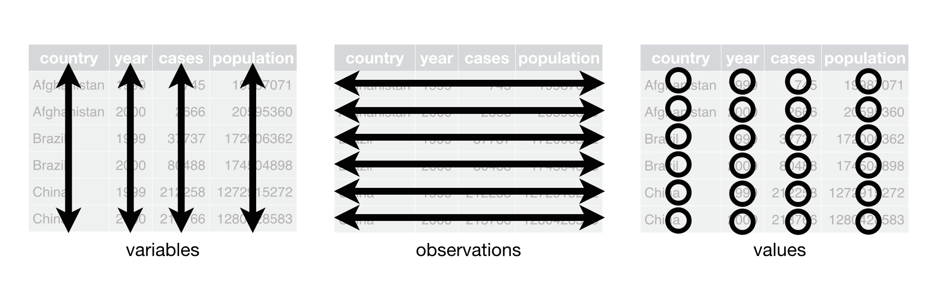
Tidy data is a standard way of organizing tables that makes them easier to work with. The tidy data principles are simple but powerful, and they apply to almost any kind of data.

Tidy data rule

One row per observation
One column per variable
One cell per value

Wide table: year in the column name

wide_rates <- data.frame(
  municipality_code = c("0180", "0380", "1280"),
  unemployment_rate_2022 = c(10.5, 10.2, 18.0),
  unemployment_rate_2023 = c(10.5, 9.9, 17.7)
)
wide_rates

  municipality_code unemployment_rate_2022 unemployment_rate_2023
1              0180                   10.5                   10.5
2              0380                   10.2                    9.9
3              1280                   18.0                   17.7

Tidy table: year as a variable

tidy_rates <- data.frame(
  municipality_code = c("0180", "0180", "0380", "0380", "1280", "1280"),
  year = c(2022, 2023, 2022, 2023, 2022, 2023),
  unemployment_rate = c(10.5, 10.5, 10.2, 9.9, 18.0, 17.7)
)
tidy_rates

  municipality_code year unemployment_rate
1              0180 2022              10.5
2              0180 2023              10.5
3              0380 2022              10.2
4              0380 2023               9.9
5              1280 2022              18.0
6              1280 2023              17.7

Same question, two table shapes

Both tables contain the same information, but one is easier to work with:

wide_rates[c("municipality_code", "unemployment_rate_2023")]

  municipality_code unemployment_rate_2023
1              0180                   10.5
2              0380                    9.9
3              1280                   17.7

tidy_rates[tidy_rates$year == 2023, c("municipality_code", "unemployment_rate")]

  municipality_code unemployment_rate
2              0180              10.5
4              0380               9.9
6              1280              17.7

Why tidy usually wins

Same code across years
Easier filtering
Easier joining
Easier plotting

Basic Checks

Vectors
From Vectors To Tables
Subsetting Tables
Working With Table Columns
Categories
Tidy Data
Basic Checks
Quick Inspection Plots

Check names and types

Before filtering or plotting, check the boring structure first:

names(panel_df)[1:6]

[1] "municipality_code" "municipality_name" "year"             
[4] "unemployment_rate" "high_unemployment" "period"

str(panel_df)

'data.frame':   2320 obs. of  6 variables:
 $ municipality_code: chr  "0114" "0115" "0117" "0120" ...
 $ municipality_name: chr  "Upplands Väsby" "Vallentuna" "Österåker" "Värmdö" ...
 $ year             : int  2016 2016 2016 2016 2016 2016 2016 2016 2016 2016 ...
 $ unemployment_rate: num  11.9 6.1 7.2 7.3 13.7 5.6 12 17.7 9.7 11.9 ...
 $ high_unemployment: logi  TRUE FALSE FALSE FALSE TRUE FALSE ...
 $ period           : chr  "older" "older" "older" "older" ...

Names reveal variable content
Types reveal how R will treat the column

Check the range

Summary statistics catch implausible values quickly:

summary(panel_df$unemployment_rate)

   Min. 1st Qu.  Median    Mean 3rd Qu.    Max. 
   5.00    9.80   12.20   12.49   14.80   23.40

Minimum and maximum
Center and spread
Anything implausible?

Check missing values

Then count missingness explicitly:

sum(is.na(panel_df$unemployment_rate))

[1] 0

Missing values?
Count first
Investigate next

Check the key

any(duplicated(panel_df[c("municipality_code", "year")]))

[1] FALSE

head(panel_df[c("municipality_code", "year")])

  municipality_code year
1              0114 2016
2              0115 2016
3              0117 2016
4              0120 2016
5              0123 2016
6              0125 2016

Break the table on purpose

bad_panel <- panel_df[c(1, 2, 3, 4, 1), ]
bad_panel$unemployment_rate[2] <- NA

One missing value
One duplicated key

Check the broken example

is.na(bad_panel$unemployment_rate)

[1] FALSE  TRUE FALSE FALSE FALSE

duplicated(bad_panel[c("municipality_code", "year")])

[1] FALSE FALSE FALSE FALSE  TRUE

any(duplicated(bad_panel[c("municipality_code", "year")]))

[1] TRUE

Filter out missing rows

bad_panel[!is.na(bad_panel$unemployment_rate), ]

    municipality_code municipality_name year unemployment_rate
1                0114    Upplands Väsby 2016              11.9
3                0117         Österåker 2016               7.2
4                0120            Värmdö 2016               7.3
1.1              0114    Upplands Väsby 2016              11.9
    high_unemployment period
1                TRUE  older
3               FALSE  older
4               FALSE  older
1.1              TRUE  older

Keep observed rows
Drop missing values explicitly

Checklist for a new table

Row meaning
Key
Unique key?
Right types?
Missing values?

Quick Inspection Plots

Vectors
From Vectors To Tables
Subsetting Tables
Working With Table Columns
Categories
Tidy Data
Basic Checks
Quick Inspection Plots

Why plot now?

Simple plots are useful long before polished visualization:

Check data fast
Use in problem sets
Better design in lecture 10

Three quick plot patterns

hist(x)
boxplot(x)
plot(x, y)

Histogram

hist(
  panel_df$unemployment_rate,
  breaks = 30,
  main = "Municipal unemployment rates",
  xlab = "Unemployment rate"
)

Quick boxplot

recent_panel <- subset(panel_df, year >= 2020)
boxplot(
  formula = unemployment_rate ~ year,
  data = recent_panel,
  xlab = "Year",
  ylab = "Unemployment rate"
)

Quick scatterplot

plot(
  x = panel_df$year,
  y = panel_df$unemployment_rate,
  xlab = "Year",
  ylab = "Unemployment rate"
)

Main takeaways

Vectors support element-wise work
Vectorization often avoids explicit repetition
Tables are lists of equal-length vectors
Keys and identifiers matter
Tidy helps repeated work
Check early
Plot early