Lecture 3: R Basics I

Adam Altmejd

adam.altmejd@su.se

The Institute for Evaluation of Labour Market and Education Policy (IFAU)

2026-04-07

Why code instead of spreadsheet surgery?

 

The paper captures a common problem with spreadsheet workflows: once many manual edits accumulate, the data pipeline becomes hard to inspect, explain, and reproduce. In this case, Excel rewrote certain gene codes into dates without warnings, which led to widespread errors in the genetic literature.

Programming fundamentals

Most languages revolve around a small set of ideas:

• Expressions return values
• Operators combine values
• Assignment binds names
• Types shape behavior
• Logic builds conditions
• Control flow directs execution
• Functions package reusable code

These ideas recur across most programming languages. The syntax changes, but the underlying concepts around values, names, types, logic, and functions are broadly transferable.

Setup check

• VSCode R interpreter running
• R Script file open
• Ctrl/cmd+enter sends line to interpreter

The key distinction is conceptual: code is written in the script editor and sent to the R interpreter. In VS Code, the interpreter may run inside a terminal pane, but that pane is only the interface, not the shell itself.

I’ve been testing out Positron and it seems to work well enough by now that I actually want to recommend you to try it. Lots of R features will “just work”.

Moving from Stata to R

Some habits carry over; some do not:

• Not limited to one dataset in memory
• Stata commands = R functions
• Less “hand-holding”, need to be more mindful about what you run
• More dependent on external packages

The main transfer from Stata is conceptual rather than syntactic. Many familiar tasks still exist, but R makes objects, function calls, scripts, and packages much more explicit.

R fundamentals

“Everything that exists is an object. Everything that happens is a function call.”

All objects can be named, inspected, and reused.

This slogan, attributed to John Chambers (the creator of the S language), is informal, but useful. In R, values, tables, functions, and model results are all objects that can be named, inspected, stored, and passed to other functions.

Expressions, Operators, And Assignment

• Expressions, Operators, And Assignment

• Objects And Types

• Logic And Missingness

• Control Flow

• Functions

• Packages, Comments, Errors, and Help

Arithmetic with operators

Type these in the R interpreter:

12 + 3

[1] 15

8 - 33

[1] -25

20 / 3

[1] 6.666667

10^(2 + 1) - 1

[1] 999

+, -, /, and ^ are arithmetic operators.

The R interpreter evaluates each expression and prints the resulting value. At this stage, the value is visible, but not stored under a reusable name.

Evaluation in the interpreter

• The code is an expression
• The interpreter evaluates it
• The printed result is a value
• Nothing saved yet

This is the basic rhythm of interactive work in R: type an expression, let the interpreter evaluate it, inspect the result, and decide whether it is worth storing under a name.

Assignment

<- stores an object in memory and binds a name to it

coffee_cups <- 3
price_per_cup <- 25

We can then run operations on those names:

coffee_cups * price_per_cup

[1] 75

The key idea is that values exist independently of names. Assignment connects a name to the current value in memory.

You can also use = for assignment in R, but <- is the convention. The main reason is that = is also used for naming function arguments, so <- keeps the two uses visually distinct. However, <- for assignment can also cause confusion: a < -5 (comparison to -5) and a <- 5 (assignment) look similar but do very different things.

Naming rules

• Must start with a letter
• Are case sensitive (income and Income are different)
• Descriptive beats short (no character limit!)

v1 <- 100 # valid but not descriptive
annual_income <- 100 # valid and descriptive

1a <- 1 # invalid

Error in parse(text = input): <text>:1:2: unexpected symbol
1: 1a
     ^

Names can be rebound / overwritten

result <- 3
result

[1] 3

result <- "pass"
result

[1] "pass"

Rebinding changes what the name points to; it does not mutate some permanent meaning attached to the name itself. That is why the same name can later refer to a number, a string, a table, or a function.

Reserved words

Assigning a value to these names will not work:

if
else 
while 
for
TRUE 
FALSE 
NULL 
Inf 
NaN 
NA 

or:

function <- 1

Error in parse(text = input): <text>:1:10: unexpected assignment
1: function <-
             ^

For a full list of reserved names, see here.

Predefined words

Some words are in use, but not strictly reserved:

pi

[1] 3.141593

pi <- 20
pi

[1] 20

Lots of names are already taken by built-in objects and functions.

if (T) "yes" else "no"

[1] "yes"

T <- 0
if (T) "yes" else "no"

[1] "no"

Don’t overwrite them.

T is short for TRUE, but unlike TRUE it is not reserved. If you assign T <- 0, then T no longer means TRUE, which can lead to very confusing bugs. The same goes for F and FALSE.

Session memory is temporary

• Objects live in session memory
• Restart R -> gone
• Scripts recreate state

This is one reason scripts matter. A script records how objects are created so the session can be rebuilt from code rather than from memory.

Objects And Types

• Expressions, Operators, And Assignment

• Objects And Types

• Logic And Missingness

• Control Flow

• Functions

• Packages, Comments, Errors, and Help

Objects, names, functions

Much R code can be read as a sequence of steps:

• Create or retrieve an object
• Bind it to a name
• Pass it to a function
• Get back another object
• Inspect when unsure

This is a compact reading rule rather than a complete theory of R. It is useful because many lines can be understood as: create an object, bind it to a name, pass it to a function, and get another object back.

Example

score <- 62
sqrt(score)

[1] 7.874008

• score is a name
• 62 creates a numeric object (a double)
• <- binds that object to the name score
• sqrt is a function object
• sqrt(score) calls that function

This is the recurring pattern for the course. In R, a function name like mean refers to an object. Adding parentheses, as in mean(x), calls that function with an input (the object named x).

How is an object stored in memory?

• typeof() tells us

typeof(1.0)

[1] "double"

typeof(1L)

[1] "integer"

typeof(TRUE)

[1] "logical"

typeof("text")

[1] "character"

Remember: everything is an object!

typeof(typeof)

[1] "closure"

typeof() reports the underlying storage mode of an object. This matters because the storage type influences which operations are possible and how coercion behaves later.

Basic atomic types

Most beginner examples use a few basic storage types:

• double numbers with decimals
• integer whole numbers
• logical true / false
• character text

These storage types matter because they determine which operations are valid and how values behave in vectors and tables.

typeof() is storage, class() is behavior

Storage type and class often overlap, but not always:

today <- as.Date("2026-04-07")
typeof(today)

[1] "double"

class(today)

[1] "Date"

• typeof() = how it’s stored in memory
• class() = what it does

The storage type tells how the object is represented internally, while the class tells which methods and behaviors are attached to it. Dates are a good example: stored as numbers underneath, but treated as dates by many functions.

Function methods depend on class

The same function name can behave differently for different object classes:

mean(c(1, 2, 3, 4))

[1] 2.5

mean(as.Date(c("2024-01-01", "2025-01-01")))

[1] "2024-07-02"

• Same function name
• Different object classes
• Different methods behind the scenes

This is one reason class matters in R. Many functions are generic: the printed name stays the same, but the method used depends on the class of the object supplied. Check with methods(mean) to see which methods are available for mean. Here we used mean.default() for the numeric vector and mean.Date() for the date vector.

Logic And Missingness

• Expressions, Operators, And Assignment

• Objects And Types

• Logic And Missingness

• Control Flow

• Functions

• Packages, Comments, Errors, and Help

Logic uses operators

We often need conditions, not just calculations:

1 == 2

[1] FALSE

1 < 2

[1] TRUE

1 == 2 & 1 < 2

[1] FALSE

1 == 2 | 1 < 2

[1] TRUE

• ==, <, > compare
• &, | combine conditions

Assignment is different from comparison although the symbols look similar. = assigns an object to a name, == compares two objects. Logical operators like & and | combine logical values, not numbers. The result of a logical expression is always TRUE or FALSE.

Precedence

Let’s say we want to check if a variable is larger than two other variables:

x <- 3; y <- 1; z <- 4
x > y & z

[1] TRUE

Logical operators (>, ==, etc) are evaluated before Boolean (& and |).

3 > 1

[1] TRUE

TRUE & 4

[1] TRUE

To get it right we need to be explicit:

x > y & x > z

[1] FALSE

Logical operators bind tighter than Boolean operators, so x > y & z is parsed as (x > y) & z, not x > (y & z). The second operand z (which is 4) is then coerced to logical: R runs as.logical(4), and all non-zero numbers become TRUE, only 0 becomes FALSE. This is a common source of bugs when the intended logic is not made explicit.

Decimal comparisons need care

Decimal numbers are stored as floating points (double), which can lead to surprising results:

0.3 == 0.3

[1] TRUE

0.1 + 0.2 == 0.3

[1] FALSE

Use a tolerance-based check instead:

isTRUE(all.equal(0.1 + 0.2, 0.3))

[1] TRUE

abs((0.1 + 0.2) - 0.3) < 1e-8

[1] TRUE

This is not an R quirk; it is a general feature of floating-point arithmetic in modern programming languages. Equality checks on decimal numbers can therefore fail even when two values look the same when printed.

! negates a logical result

! flips TRUE to FALSE and FALSE to TRUE:

!TRUE

[1] FALSE

!(1 < 3)

[1] FALSE

• Useful for “not”
• Common in filters

Not available = NA

NA is a missing value indicator

• NA is not zero
• NA is not false
• NA is not equal to itself!

NA > 0

[1] NA

NA == FALSE

[1] NA

NA == NA

[1] NA

Unlike Stata, missing values are not treated as very large numbers. Missingness often propagates through calculations until it is handled explicitly.

NA could be anything

Missingness propagates through logical operations:

NA > 0

[1] NA

NA & TRUE

[1] NA

But:

NA | TRUE

[1] TRUE

NA & FALSE

[1] FALSE

Here, it does not matter what NA could be, since both TRUE | TRUE and FALSE | TRUE evalute to TRUE.

is.na() checks missingness

is.na() returns TRUE for missing values:

• TRUE means missing
• FALSE means observed

is.na(NA)

[1] TRUE

is.na(3)

[1] FALSE

is.na() is the standard way to test for missingness. On longer objects it returns one logical result per element; that becomes especially important when working with vectors and tables.

Special values in numeric work

Some numeric operations do not return ordinary finite numbers or NA:

• Inf / -Inf from dividing by zero
• NaN from undefined numeric operations

1 / 0

[1] Inf

0 / 0

[1] NaN

is.na() catches both NA and NaN, use is.nan() to catch only NaN:

is.na(NaN)

[1] TRUE

is.nan(NA)

[1] FALSE

is.nan(NaN)

[1] TRUE

These values are easy to confuse, but they mean different things. NA means a value is missing, while NaN means a numeric calculation itself was undefined.

Control Flow

• Expressions, Operators, And Assignment

• Objects And Types

• Logic And Missingness

• Control Flow

• Functions

• Packages, Comments, Errors, and Help

Control flow decides what runs

• Logic creates conditions
• Control flow uses them
• Branch or repeat as needed

Without control flow, code runs from top to bottom in a fixed order. Control-flow tools make execution depend on conditions or repetition, which is what turns isolated expressions into small programs.

if / else

Use if / else when one logical value should choose one branch:

if (condition) "do this" else "do that"

condition is a single logical value that determines which expression is evaluated and returned.

if (1 == 3) "foo" else "bar"

[1] "bar"

if / else is a control-flow tool: the result depends on whether a condition evaluates to TRUE or FALSE. The important restriction is that the condition must be a single logical value.

Prefer the multi-line form

if (TRUE) {
    "yes"
} else {
    "no"
}

[1] "yes"

The one-line form is valid, but the multi-line form is usually easier to read, extend, and debug. Braces and line breaks matter more once conditions and returned expressions become longer.

for loops repeat a block

for (i in 1:4) {
    print(i^2)
}

[1] 1
[1] 4
[1] 9
[1] 16

• Repeats one recipe
• i takes one value at a time
• Basic control-flow tool

A for loop runs the same block repeatedly while a name takes different values in turn. Here 1:4 is a short way to generate the sequence from 1 to 4.

Functions

• Expressions, Operators, And Assignment

• Objects And Types

• Logic And Missingness

• Control Flow

• Functions

• Packages, Comments, Errors, and Help

Why functions matter

Functions make code more reusable:

• Same recipe, new inputs
• Less repetition
• Easier testing
• Easier debugging

Functions package a small piece of logic so it can be reused with different inputs. This is one of the main ways programming scales beyond one-off commands typed directly into the interpreter.

Functions: inputs and output

A function call passes inputs to a function and returns an object:

sqrt(16)

[1] 4

abs(-12)

[1] 12

round(pi)

[1] 3

When a function is called, R evaluates the call and produces a result. Result can be printed or just stored. In simple cases it helps to think of the arguments being matched to the function’s parameter names and the function body then being evaluated with those values.

Function call structure

round(pi, digits = 3)

[1] 3.142

• round is the function
• pi is the first argument
• digits = 3 names another argument
  • digits is an optional argument with a default of 0
• The call returns 3.142
• The return value is printed

This example separates five ideas that are easy to blur together: the function object itself, the values passed in, the names of optional arguments, and the value returned by the call. That distinction carries over directly to other programming languages.

Functions are objects too

typeof(mean)

[1] "closure"

class(mean)

[1] "function"

Functions are ordinary objects in R: they can be inspected, named, stored, and then called with arguments.

Creating a function

function() creates a new function object:

add_bonus <- function(score, bonus = 5) {
    score + bonus
}

• Name on the left
• Arguments inside function(...)
• Returned expression inside { ... }

The function definition creates a new function object and stores it under the name add_bonus. When the function is called, score and bonus are bound to the supplied arguments, and the expression inside the body is evaluated. Here the returned value comes from the last expression, score + bonus.

Named and default arguments

Inside function calls = names an argument.

Functions can also provide defaults:

add_bonus <- function(score, bonus = 5) {
    score + bonus
}

add_bonus(55)

[1] 60

add_bonus(55, bonus = 10)

[1] 65

Default arguments make a function easier to reuse because common choices do not have to be repeated every time. Naming an argument inside the call makes it explicit which parameter is being changed.

Arguments

Myfunc takes two arguments, v1 and v2, and returns the larger of the two. v2 has a default value of 5, so if it is not supplied, the function will compare v1 to 5.

myfunc <- function(v1, v2 = 5) {
    max(v1, v2)
}

myfunc(1,2)

[1] 2

myfunc(1,2,3)

Error in `myfunc()`:
! unused argument (3)

myfunc(c(1,2))

[1] 5

The last call returns 5 and not 2 because the whole c(1,2) is supplied for v1 and no object is supplied for v2.

Scoping: functions use “local” names

x <- 10
show_local <- function() {
    x <- 20
    x
}
c(show_local(), x)

[1] 20 10

• Function call creates local names
• Local assignment stays local
• Outer name unchanged

x <- 10 assigns 10 to the name x in the global environment. In a sense, all global environment objects are like “globals” in Stata. When show_local() runs, it creates a new local name x that is separate from the global x. The assignment x <- 20 changes the local x, but does not affect the global x.

Where does R look for a name?

x <- 10
add_outer_x <- function(z) {
    z + x
}
add_outer_x(5)

[1] 15

• Function arguments and local names first
• Then surrounding names
• If still missing: object 'name' not found
• Convenient but bug prone
  • Pass all used objects as arguments

R first looks for a name inside the function call itself, then outward to surrounding environments. That is useful, but it also creates a common failure mode: code silently depends on an outer object that was never passed as an argument, or errors because the author assumed a name would already exist.

You need to tell R where to look

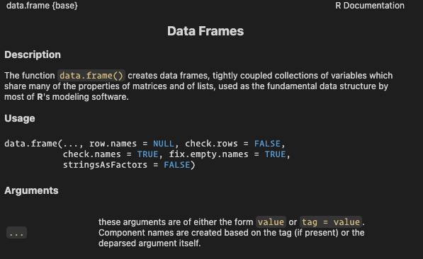
toy_df <- data.frame(
    x = c(1, 2, 3),
    y = c(2, 4, 5)
)

lm(y ~ x)

Error:
! object 'y' not found

coef(lm(y ~ x, data = toy_df))

(Intercept)           x 
  0.6666667   1.5000000 

• x and y are column names inside toy_df
• lm(y ~ x) looks for objects named x and y
• data = toy_df tells R where to look

A common error, especially when coming from Stata. The formula uses the column names, but those names live inside the table rather than in the global environment. Passing data = toy_df tells the function to evaluate the formula inside that data frame instead of in the global environment.

Packages, Comments, Errors, and Help

• Expressions, Operators, And Assignment

• Objects And Types

• Logic And Missingness

• Control Flow

• Functions

• Packages, Comments, Errors, and Help

Packages extend R

Packages add functions, datasets, and tools:

install.packages("ggplot2")
library(ggplot2)

• Install once
• Load when needed
• Read package documentation

Base R already does a lot, but packages are a central part of the language. Most real projects use a mix of base functions and contributed packages.

package::function() syntax

This pattern makes the source of a function explicit:

readr::read_csv("data.csv")
stats::filter(x, rep(1 / 3, 3))

• Avoid name conflicts
• Clarify provenance

Different packages can export functions with the same name. Writing package::function() avoids ambiguity and makes it clear which implementation is being used.

Comments start with #

Comments are text for humans. The interpreter ignores them:

# myfunc(x, y) returns largest number of v1 and v2
myfunc = function(v1, v2) max(v1, v2)

• Add intent
• Add context
• Add warnings when needed
• Use comments to get code suggestions from Copilot

But: “Good code explains itself”

return_largest_number = function(v1, v2) max(v1, v2)

Comments are useful when they explain intent, assumptions, or gotchas that are not obvious from the code itself. They are not part of the computation.

Prefer comments that add context

# Less helpful:
# Calculate the mean
m <- mean(x, na.rm = TRUE)

# Better:
average_non_missing <- mean(x, na.rm = TRUE)

• Clear names first
• Comments for context
• Avoid narrating obvious code

Self-explanatory names do most of the work. Comments are most useful when they explain why something is done, not simply what a line already says.

Pipes (|>) make code easier to read

mean(c(seq(0, 10), rep(NA, 10)), na.rm = TRUE)

[1] 5

is the same as

seq(0, 10) |> 
  append(rep(NA, 10)) |> 
  mean(na.rm = TRUE)

[1] 5

• Piped content enters the first argument of the next function
• Avoids nested parentheses
• Reads left to right
• Still a function call, just different syntax

A quick intro to figuring out what went wrong

• Read the error
• Check names
• Print object
• Check type / class
• Get help

We’ll cover debugging in more depth later, but these are the main steps to take when an error occurs. The key is to read the error message carefully and then use tools like exists(), printing, and checking types to understand what went wrong.

Read the error

my_data <- data.frame(a = c(1, 2), b = c(3, 4))
my_dat[1]

Error:
! object 'my_dat' not found

• my_data exists
• my_dat does not

The important habit is to read the error literally before guessing at a fix. In this example the problem is not indexing syntax or object type; it is simply that the name in the second line does not match the name that was created.

Understand the error

dat = data.frame(a = c(1,2),
                 b = c(3,4))
data[1]

Error in `data[1]`:
! object of type 'closure' is not subsettable

!?!?

typeof(data)

[1] "closure"

typeof(dat)

[1] "list"

Learning to read error messages will help you find coding errors.

Talk on this famous error: https://posit.co/resources/videos/object-of-type-closure-is-not-subsettable/

Check names

exists("my_data")

[1] TRUE

exists("my_dat")

[1] FALSE

• Exact spelling matters
• One letter can break the code

Many early errors are simple naming problems. Before changing code, check whether the object name being used actually exists in memory.

Print object

my_data

  a b
1 1 3
2 2 4

• Check visible values
• Check obvious surprises

Printing the object is often the fastest way to catch a wrong value, a wrong shape, or a mistaken assumption about what the object contains.

Check type / class

typeof(my_data)

[1] "list"

class(my_data)

[1] "data.frame"

• Storage and behavior both matter
• Different objects support different operations

An expression may fail simply because the object is not the kind of thing the code expects. Checking both typeof() and class() helps narrow that down.

Get help

• ?mean
• ?data.frame
• args(mean)
• example(plot)

 

Help pages describe what a function does, what arguments it accepts, and what kind of object it returns. args() is a quick way to inspect the argument names without reading the full help page. example() runs the examples from a help page, which is often a fast way to see a function in action.

Package docs and vignettes

Package documentation is often the best starting point:

help(package = "ggplot2")
vignette(package = "ggplot2")

• Help page for the package
• List available vignettes

Function help pages answer small local questions. Vignettes are better when the goal is to understand a package’s overall workflow, conventions, and typical usage patterns.

Main takeaways

• Expressions return values
• Assignment creates reusable names
• Types shape behavior
• Logic is explicit
• Control flow shapes execution
• Functions package reusable work
• Packages extend the language
• Help and errors are part of the workflow

Next lecture: Vectors, Tables, and Tidy Thinking