Lecture 10: Visualization and Communication

Adam Altmejd

adam.altmejd@su.se

The Institute for Evaluation of Labour Market and Education Policy (IFAU)

2026-05-28

Why visualize?

The greatest value of a picture is when it forces us to notice what we never expected to see.

John Tukey, The Future of Data Analysis (1962)

Quote popularised via Tufte (1983)

Why visualize? (cont.)

• In 1854, a horrible cholera epidemic was ravaging London
• Doctors believed “miasma” (bad air) had caused the disease
• John Snow (“father of epidemiology”) argued it was transmitted through water
• But it wasn’t the study’s identification strategy that convinced people, it was its visualization

Snow (1855)

• Crazy as it sounds, people were still generally not believing in the germ theory of disease.
• Snow had many intellectual children: he is sometimes also called the father of causal inference. His water-company comparison is arguably the first DiD.

Snow’s cholera map

 

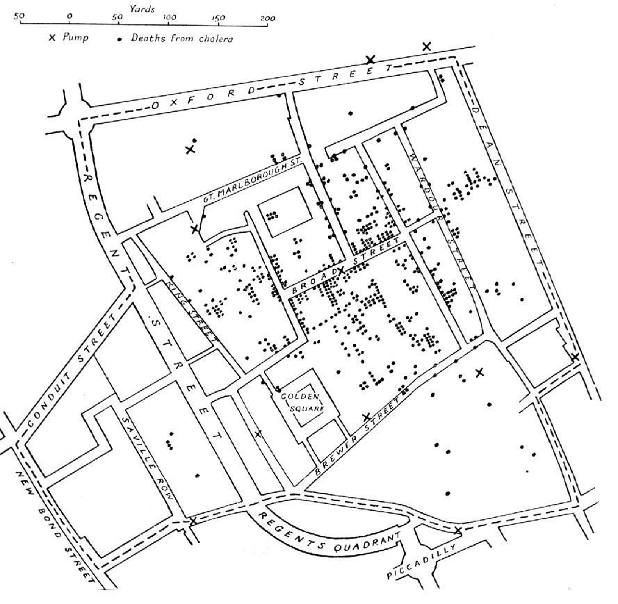
Snow (1855)

Anscombe’s quartet

dt = as.data.table(datasets::anscombe)
modelsummary::datasummary(All(dt) ~ N + mean + SD, data = dt)

	N	mean	SD
x1	11	9.00	3.32
x2	11	9.00	3.32
x3	11	9.00	3.32
x4	11	9.00	3.32
y1	11	7.50	2.03
y2	11	7.50	2.03
y3	11	7.50	2.03
y4	11	7.50	2.03

Anscombe (1973)

Anscombe’s quartet

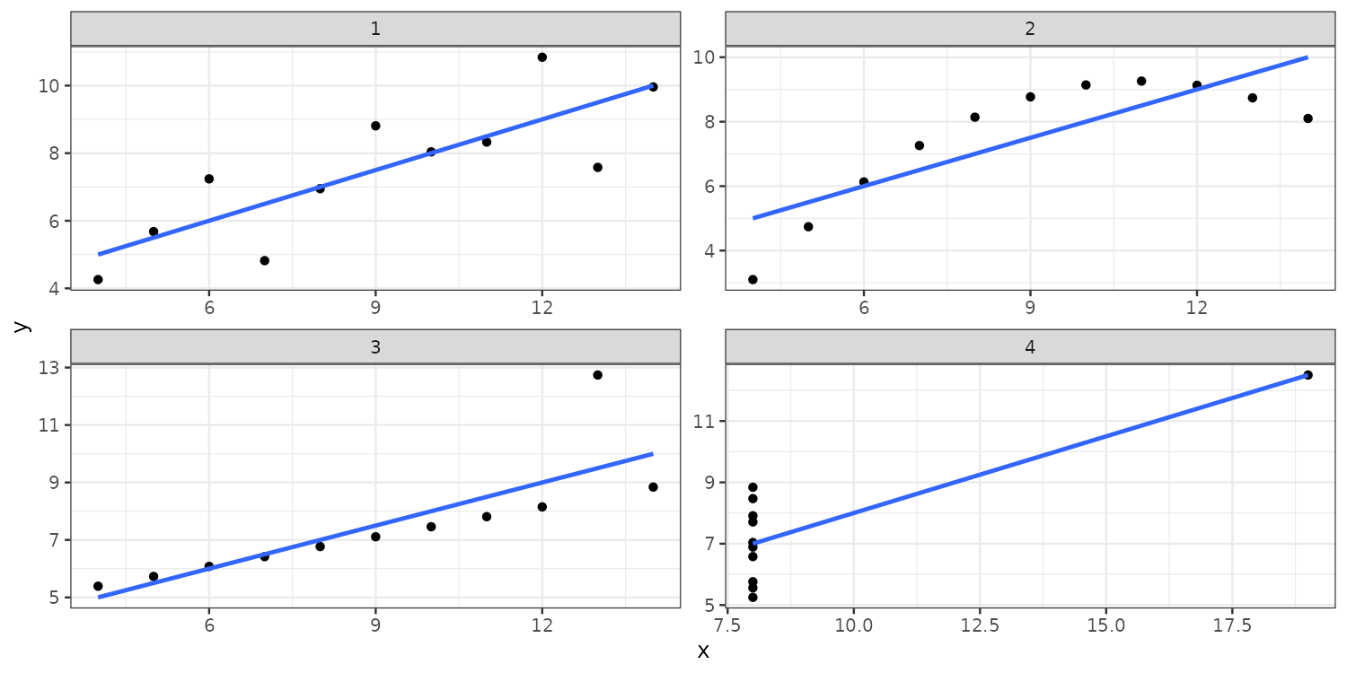
Anscombe (1973)

What visualization is for

• Summary statistics are not enough! They can hide critical patterns and differences in data.
• Visualization helps us:
  • Explore for patterns, trends, outliers, and relationships
  • Understand complex datasets more intuitively
  • Analyze insights missed by numerical methods
  • Evaluate models (e.g., residual plots)
  • Communicate findings clearly and effectively

Two modes of plotting

Exploration

• You are the audience
• Many quick plots, made fast
• Defaults are usually fine
• One question per plot is fine
• Iteration beats polish

Communication

• Someone else is the audience
• A few plots, made carefully
• Defaults rarely are
• Each plot should make one clear point
• Polish: titles, captions, framing

Same grammar, different goals. Most of this lecture is about communication.

Summary statistics hide patterns

https://janhove.github.io/posts/2016-11-21-what-correlations-look-like/

Examples: (14) is Simpson’s paradox, (15) extreme value sampling inflates r.

Test your correlation-guessing skills on https://www.guessthecorrelation.com/

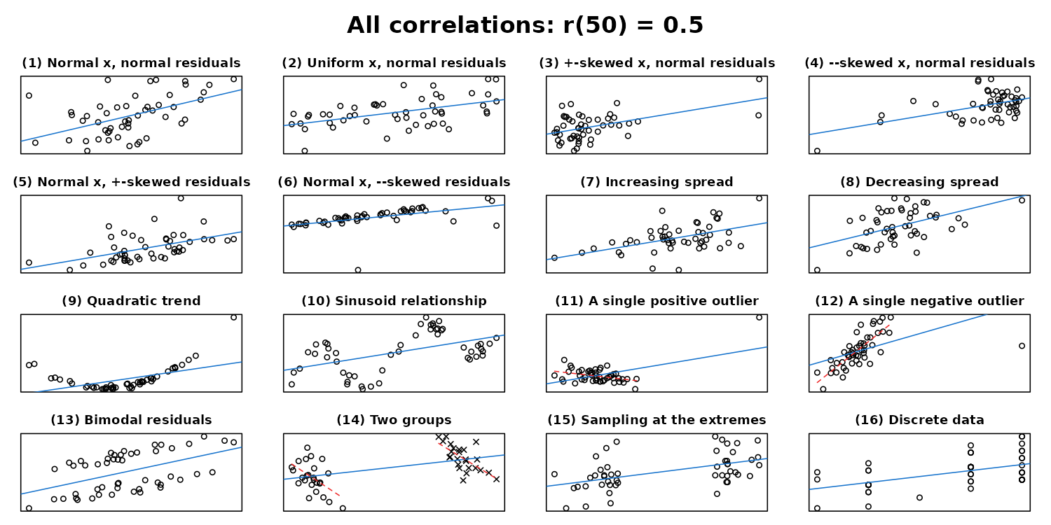
Datasaurus: same stats, different shapes

 

Matejka and Fitzmaurice (2017)

This is an animation of various data scatter patterns with identical summary statistics.

Wrangling ↔︎ Visualization

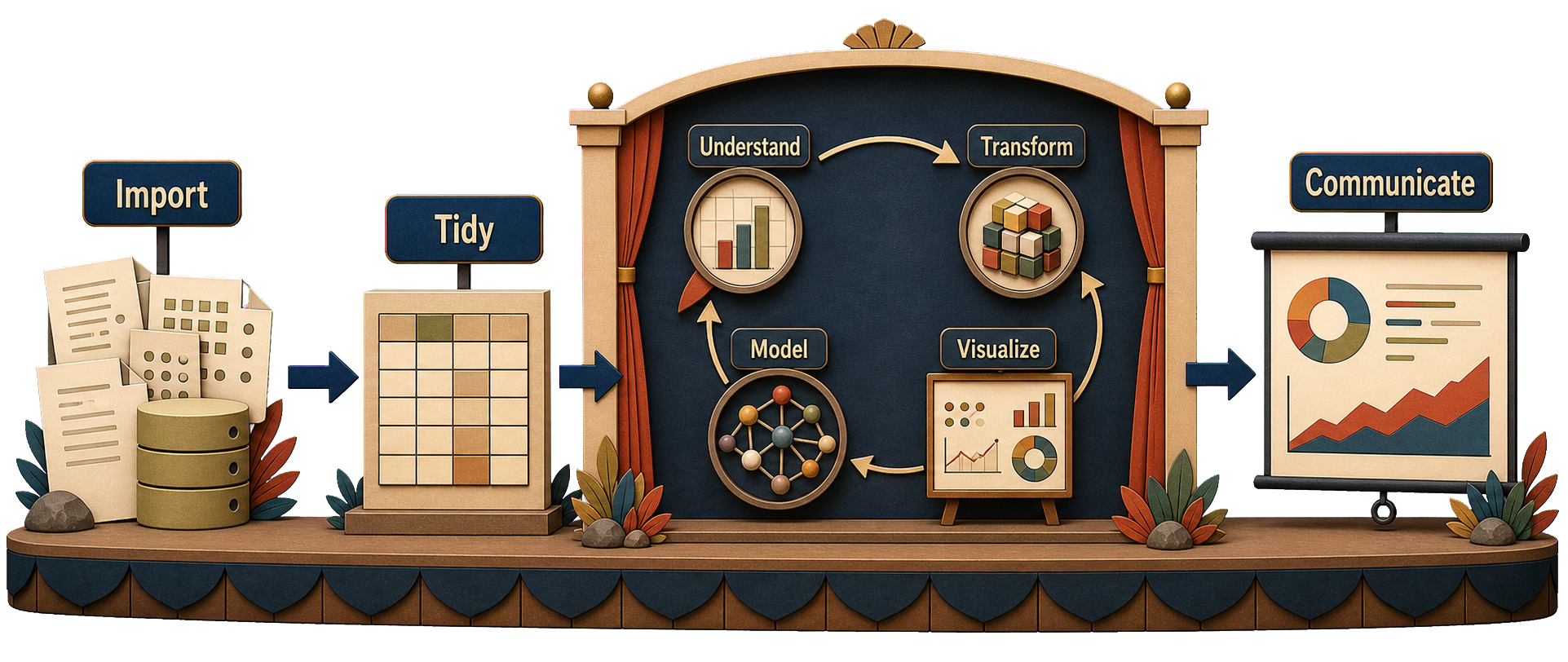
Workflow adapted from Wickham et al. (2023)

Exploring data visually is often the best way to understand it and to discover issues.

Data verification

• Some of your data will be wrong
• Finding out which and how early saves lots of time and energy
  • You don’t want to realize halfway through a project that an important category has been coded as missing.

Verification tasks:

• Browse data (using View() or just print it)
• Check descriptives: missing, unique values, mean/median/min/max
• Plot data: scatters, histograms, densities

Internal consistency: Is the data represented correctly?

• Potential sources of problems:
  • Incomplete or duplicated data
  • Missing or incorrectly coded values
  • Encoding problems

Verifying the variable wage, we might ask:

• Do the values make sense?
• Is there bunching at high-frequency values?
• Are zeros and missing coded separately?
• Does everyone classified as not working have 0 wage?

External consistency: What does the data represent?

• Potential sources of problems:
  • Bad survey questions
  • Measurement error
  • Sampling bias

Verifying the variable wage, we might ask:

• Are any government transfers included?
• How do population means compare to official statistics?
• Do correlations with related variables make sense?

External consistency example

• Researchers use health records to study public health
• Can you see the external consistency problem?

I want to study health. Health records are a (reasonably) accurate measure of health care, but a biased measure of health.

Visualization is also communication

• Figures are often the most effective way to communicate results
• Much of what you learn will be just as useful for communication

Tufte: Graphical excellence

[Graphical excellence] is that which gives to the viewer the greatest number of ideas in the shortest time with the least ink in the smallest space

Edward Tufte

Charles Minard’s Infographic of Napoleon’s Invasion of Russia (1869)

 

• “Tells a rich, coherent story with multivariate data”
• Six plotted variables: size of army, two-dimensional location, direction, temperature.

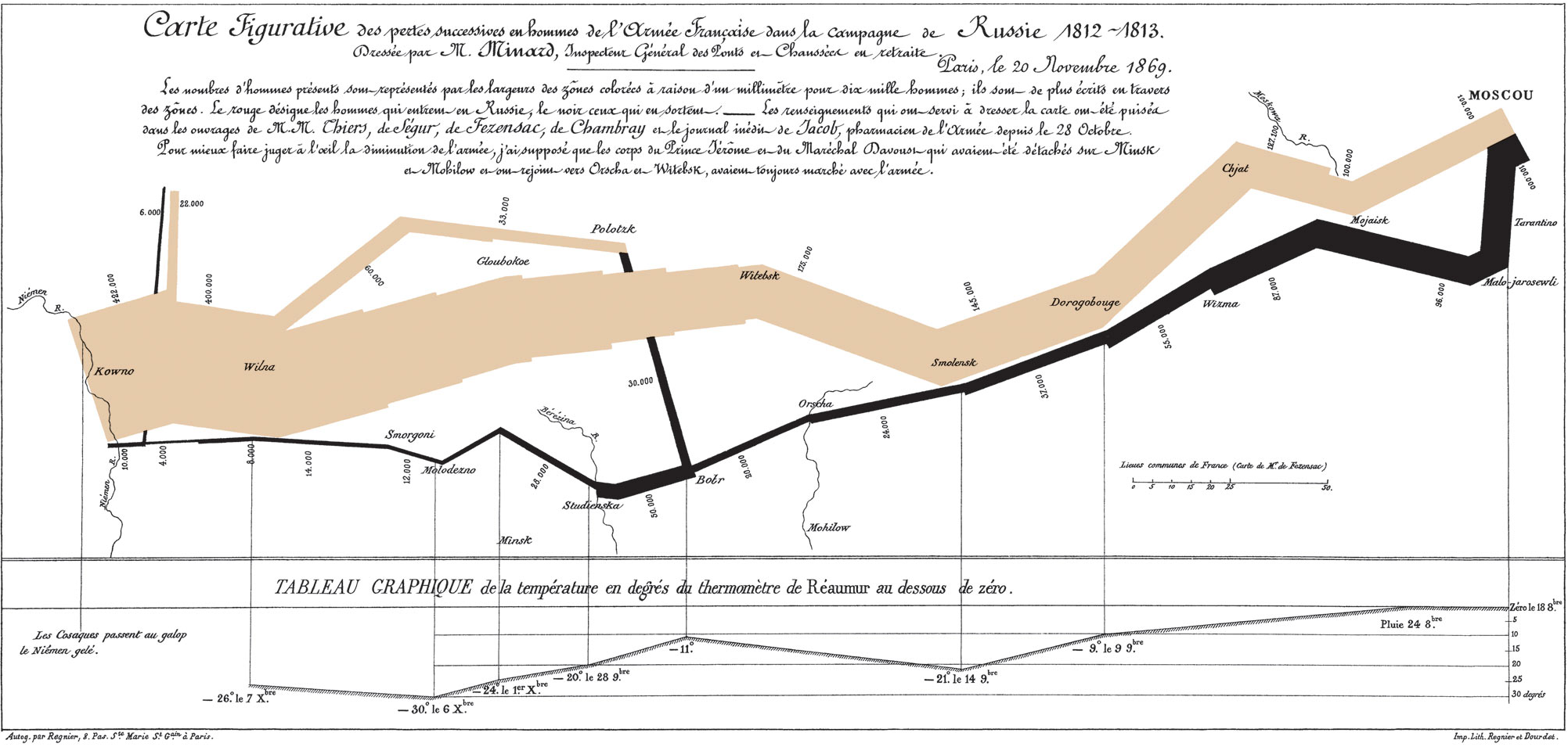
Tufte (1983)

Bad graphs: Pandemic TV edition

 

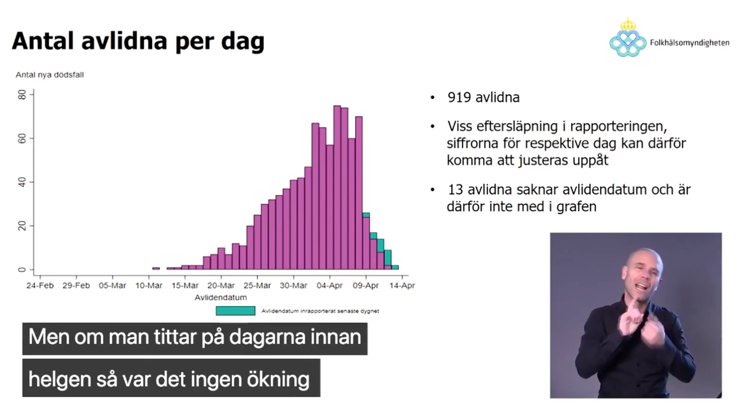
Let’s plot the FOHM data ourselves

fohm_dt <- fread(here("lectures", "lecture_10", "fohm_c19_death_data.csv"))[!is.na(date)]

ggplot(data = fohm_dt[publication_date == "2020-04-13"],
       aes(x = date, y = N)) +
  geom_col() + scale_x_date() +
  geom_vline(xintercept = as.Date("2020-04-08")) + geom_hline(yintercept = 70) + 
  coord_cartesian(xlim = as.Date(c("2020-03-01", "2020-04-30")), ylim = c(0, 120)) +
  labs(title = "Publication date: 2020-04-13", x = NULL, y = "Deaths")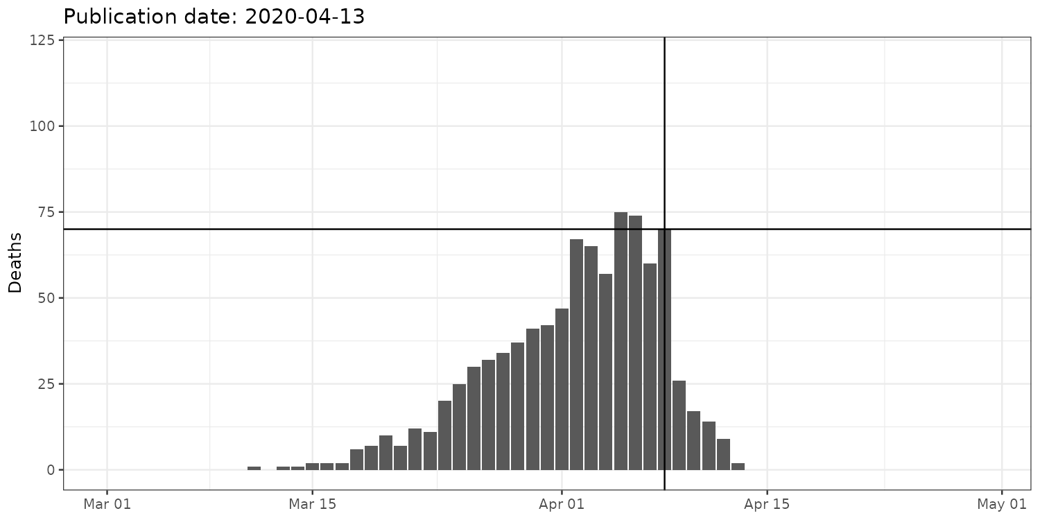

What happened then?

ggplot(data = fohm_dt[publication_date %between% list("2020-04-13", "2020-05-15")],
       aes(x = date, y = N, group = date)) +
  geom_col() + scale_x_date() +
  geom_vline(xintercept = as.Date("2020-04-08")) + geom_hline(yintercept = 70) +
  coord_cartesian(xlim = as.Date(c("2020-03-01", "2020-04-30")), ylim = c(0, 120)) +
  labs(title = "Publication date: {frame_time}", x = NULL, y = "Deaths") +
  transition_time(publication_date) + ease_aes('linear')

Same lesson, course data: spaghetti

panel_dt <- fread(here("lectures", "lecture_1", "lecture_1_demo_panel.csv"))

ggplot(panel_dt, aes(x = year, y = unemployment_rate, group = municipality_code)) +
  geom_line(alpha = 0.4) +
  labs(x = NULL, y = "Unemployment rate (%)")

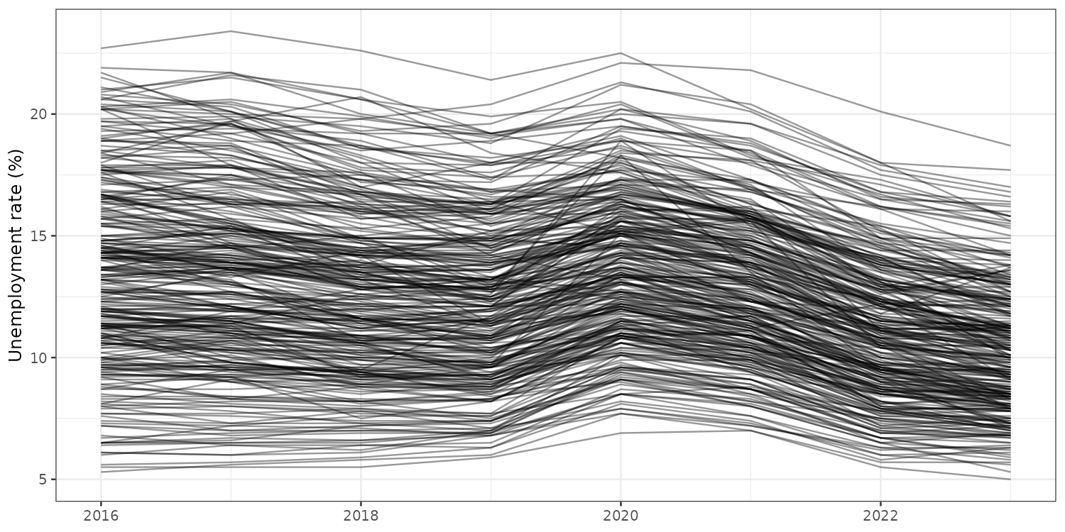
290 municipalities. You can tell rates fell, but not much else.

Same data, better figure

highlighted <- c("Danderyd", "Stockholm", "Malmö", "Pajala")

ggplot(panel_dt, aes(x = year, y = unemployment_rate, group = municipality_code)) +
  geom_line(color = "grey80", linewidth = 0.4) +
  geom_line(data = panel_dt[municipality_name %in% highlighted],
            aes(color = municipality_name), linewidth = 1.2) +
  scale_color_brewer(palette = "Dark2", name = NULL) +
  labs(x = NULL, y = "Unemployment rate (%)")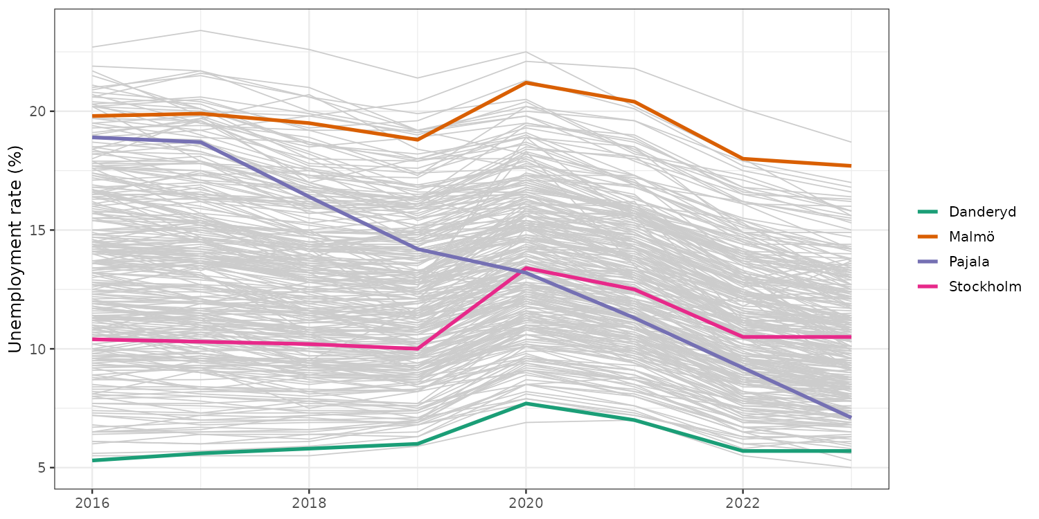

Background keeps the distribution. Foreground tells a story.

Good visualization leverages human perception

• We are good at comparing:
  • Position along a common scale
  • Length
• We are less accurate at judging:
  • Angle
  • Area/volume
  • Color intensity/shade (relative comparisons dominate)

Aspect ratios and scale

 

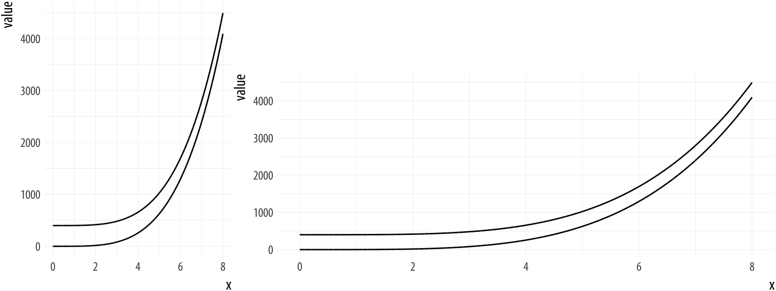
Healy (2018)

These two curves are identical, but they do not look it. The different aspect ratios of the plot affect our visual perception of how quickly the curve is changing.

Color perception is relative

 

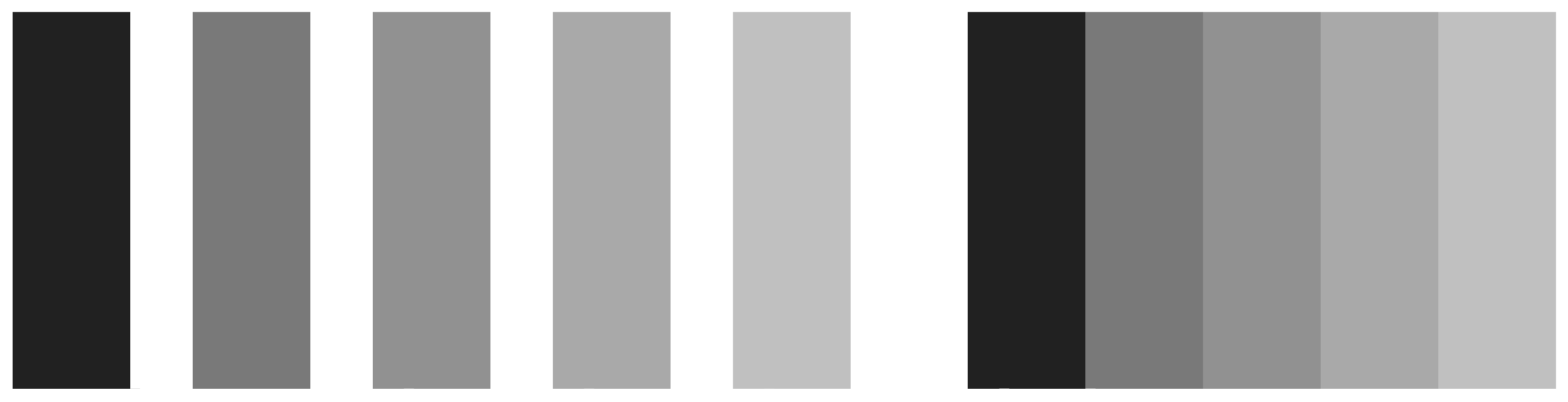
Mach bands, adapted from Healy (2018)

The brightness or luminance of the corresponding bars is the same. However, when the bars touch, the dark areas seem darker and the light areas lighter.

ggplot intro

• ggplot intro

• Plot types

• Grouping and summarizing

• Styling

• Wrapping up

Grammar of graphics

• We will learn how to make plots in R using the popular ggplot2 package
• ggplot2 implements the “grammar of graphics” graph-building paradigm
• Builds plots layer by layer, adding geometries (“geoms”)

A basic ggplot template

ggplot(data = <DATA_FRAME>,
       mapping = aes(<MAPPINGS>)) +
  <GEOM_FUNCTION>() +
  # Add more layers (optional)
  <SCALE_FUNCTION>() +
  <THEME_FUNCTION>() +
  <LABS_FUNCTION>()

Using the gapminder data

set.seed(2026)
gapminder_dt <- as.data.table(gapminder::gapminder)
tt(gapminder_dt[sample.int(nrow(gapminder_dt), 10), ])

country	continent	year	lifeExp	pop	gdpPercap
Iraq	Asia	1952	45.32000	5441766	4129.7661
West Bank and Gaza	Asia	1952	43.16000	1030585	1515.5923
Mexico	Americas	1992	71.45500	88111030	9472.3843
China	Asia	1977	63.96736	943455000	741.2375
Turkey	Europe	1992	66.14600	58179144	5678.3483
Vietnam	Asia	1962	45.36300	33796140	772.0492
Nigeria	Africa	1967	41.04000	47287752	1014.5141
Botswana	Africa	1987	63.62200	1151184	6205.8839
Paraguay	Americas	2007	71.75200	6667147	4172.8385
Cuba	Americas	1972	70.72300	8831348	5305.4453

Creating the ggplot object (cont.)

ggplot(data = gapminder_dt)

Creating the ggplot object (cont.)

p_box <- ggplot(data = gapminder_dt,
                mapping = aes(x = continent,
                              y = lifeExp))
p_box

We set the aesthetic mapping of the ggplot object to columns of the gapminder data frame.

• Notice how continent and lifeExp are not in quotes. ggplot looks inside the object given by the data argument.
• Try running str(p_box) to look at the structure of the ggplot object.

Adding a layer

p_box + geom_point()

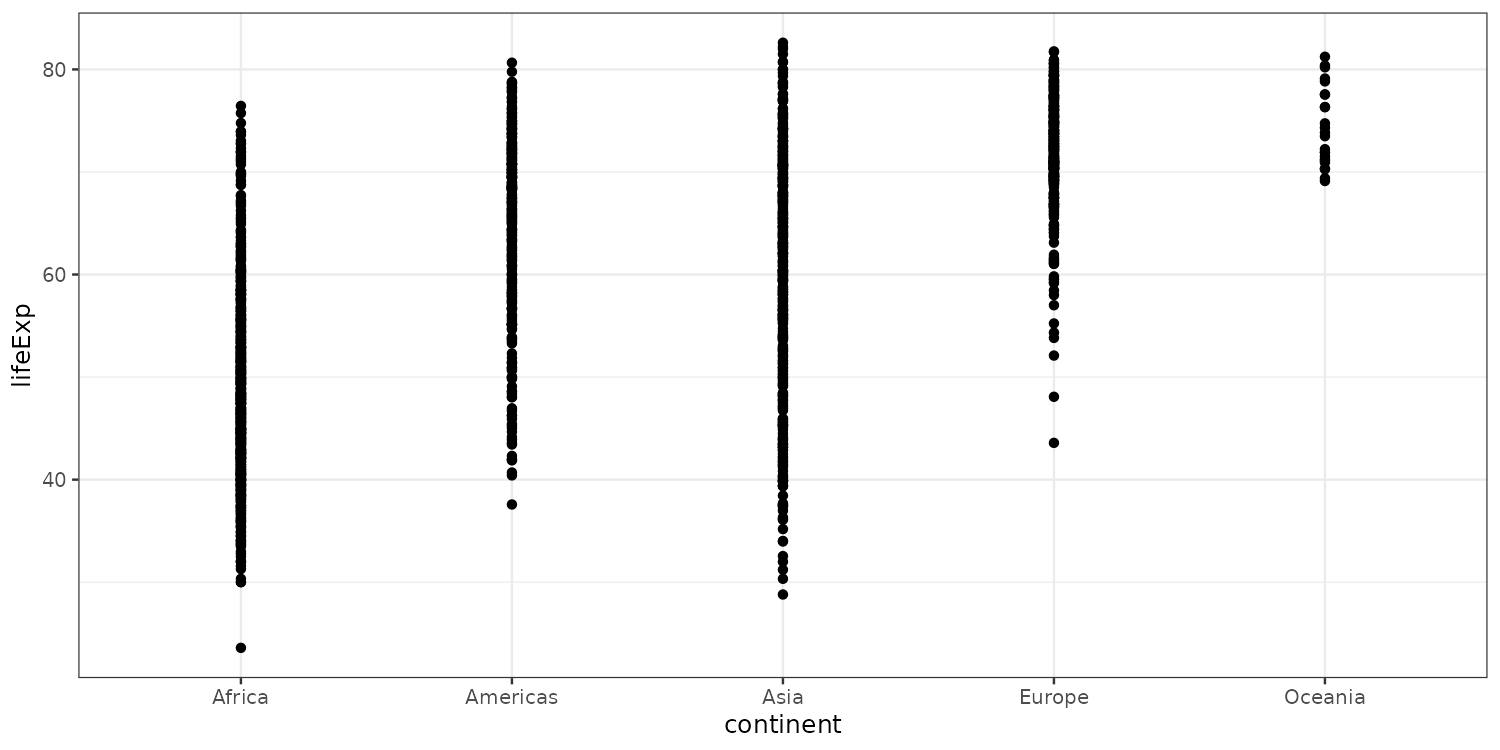
To draw something on the canvas we need to add a geometry layer. For example a scatter with geom_point().

Adding a layer (cont.)

p_box + layer(
  mapping = NULL,
  data = NULL,
  geom = "point",
  stat = "identity",
  position = "identity"
)

geom_point() is a shortcut for layer(...). Setting mapping and data to NULL means they are inherited from p_box.

Adding a boxplot

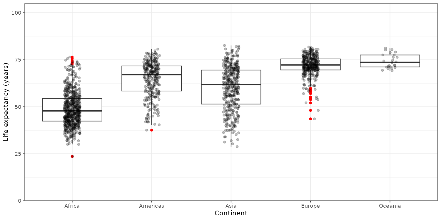
p_box + geom_boxplot()

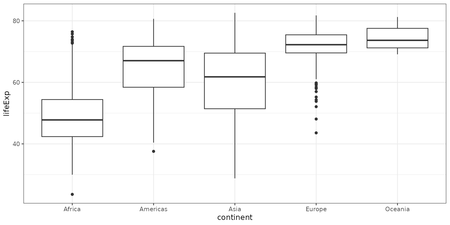
Let’s add a boxplot instead to study the distribution of continuous variables across multiple groups.

Boxplots show: median (center line), interquartile range (IQR, the box), whiskers (extending to the most extreme point within 1.5 × IQR of the box), outliers (points beyond the whiskers).

Adding another geom

p_box +
  geom_boxplot() +
  geom_jitter()

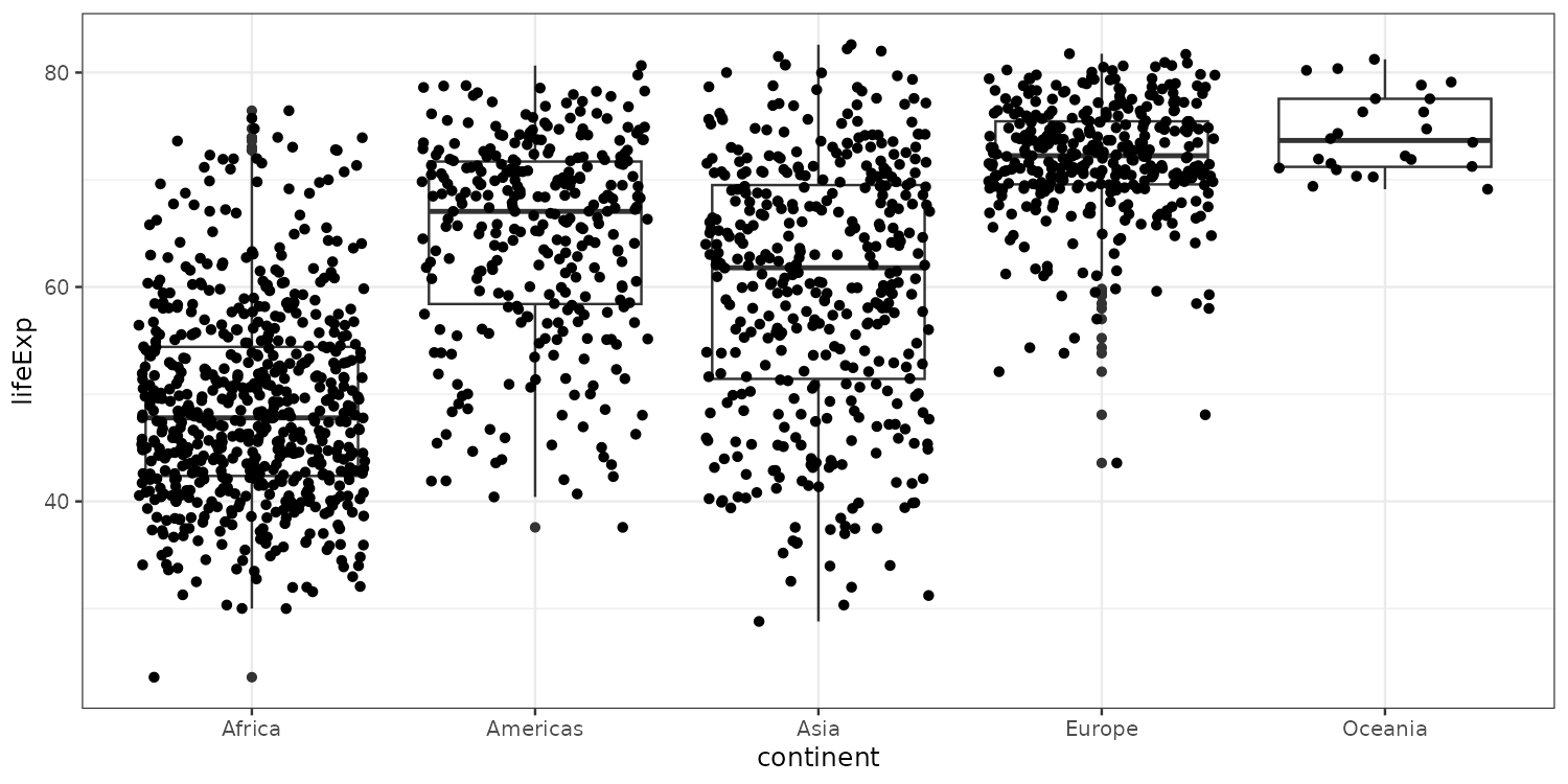
To get a more visual sense of where the data is located we can re-add the actual data points.

geom_jitter is short for geom_point(position = "jitter"). It adds a tiny bit of noise to each point so they do not overlap.

Styling geoms

p_box +
  geom_boxplot(outlier.color = "red") +
  geom_jitter(position = position_jitter(width = 0.1, height = 0),
              alpha = 0.25)

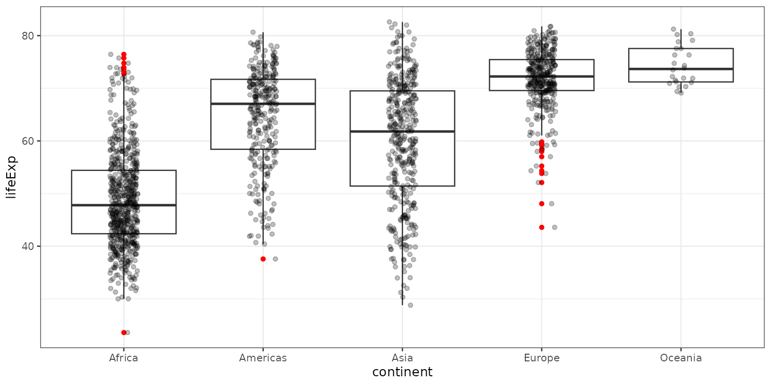
Highlighting outliers and making the points less prominent. Alpha means transparency.

Remember you can read about available function arguments by running ?geom_jitter.

Styling scales and labels

p_box +
  geom_boxplot(outlier.color = "red") +
  geom_jitter(position = position_jitter(width = 0.1, height = 0),
              alpha = 0.25) +
  scale_y_continuous(n.breaks = 5,
                     limits = c(0, 100),
                     expand = expansion(c(0,0.05))) +
  labs(y = "Life expectancy (years)",
       x = "Continent") +
  theme_bw()

Starting the y-axis at zero usually good. Here, I also added a simple theme and formatted the axis labels.

Flagging outliers

library(ggrepel)
is_outlier <- function(x) {
  x < quantile(x, 0.25) - 1.5 * IQR(x) | x > quantile(x, 0.75) + 1.5 * IQR(x)
}

plotdata <- copy(gapminder_dt)[, outlier := is_outlier(lifeExp), by = "continent"]

Tag points outside Q1 − 1.5·IQR or Q3 + 1.5·IQR per continent, then split inliers and outliers when we plot.

Labelling the outliers

p_box +
  geom_boxplot(outlier.color = "red") +
  geom_jitter(data = plotdata[outlier == FALSE],
              position = position_jitter(width = 0.1, height = 0),
              alpha = 0.25) +
  scale_y_continuous(n.breaks = 5,
                     limits = c(0, 100),
                     expand = expansion(c(0,0.05))) +
  labs(y = "Life expectancy",
       x = "Continent") +
  theme_bw() +
  geom_text_repel(data = unique(plotdata[outlier == TRUE], by = "country"),
                  aes(label = country))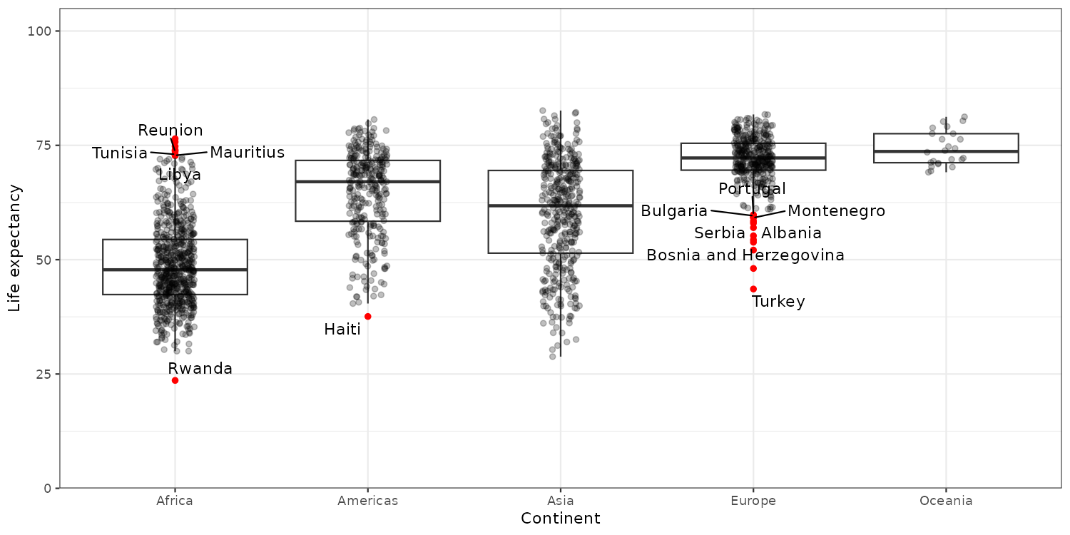

A truly powerful plotting package

• What if we want
  • To plot the relationship between GDP and life expectancy
  • Divided by countries and continents
  • To see how countries have developed over time
  • Take population size into account
• 6 dimensions 🤯
• Hans Rosling managed!

Rosling’s famous animated plot

library(gganimate)

ggplot(copy(gapminder_dt)[continent != "Oceania", ],
       aes(x = gdpPercap, y = lifeExp, size = pop, color = country)) +
  geom_point(alpha = 0.6, show.legend = FALSE) +
  scale_size(range = c(2, 13)) +
  scale_x_log10(limits = c(150, 115000),
                labels = scales::comma) +
  facet_wrap(vars(continent)) +
  coord_fixed(ratio = 1 / 43) +
  labs(title = 'Year: {frame_time}',
       x = 'GDP per capita', y = 'Life expectancy') +
  theme_minimal() +
  transition_time(year) +
  ease_aes('linear')

Rosling’s famous animated plot

Plot types

• ggplot intro

• Plot types

• Grouping and summarizing

• Styling

• Wrapping up

Common plots

• Scatter Plots (geom_point): relationships
• Line Charts (geom_line): time series
• Bar Charts (geom_col): comparisons
• Histograms & Density Plots (geom_histogram, geom_density): distributions
• Box Plots (geom_boxplot): grouped distributions
• Statistical summaries (geom_smooth, geom_errorbar): presenting results

An example dataset

Lets start by working with a really simple dataset with two groups:

df <- data.frame(
  x = c(1, 3, 4, 10, 8, 9, 3, 1, 5, 2),
  y = c(2, 6, 1, -4, 5, 1, 2, 3, 0, 4),
  gr = c(rep("a", 5), rep("b", 5))
)
df

    x  y gr
1   1  2  a
2   3  6  a
3   4  1  a
4  10 -4  a
5   8  5  a
6   9  1  b
7   3  2  b
8   1  3  b
9   5  0  b
10  2  4  b

p_xy <- ggplot(data = df,
               mapping = aes(x=x, y=y))

Individual geoms: geom_point()

p_xy + geom_point()

Individual geoms: geom_col()

p_xy + geom_col()

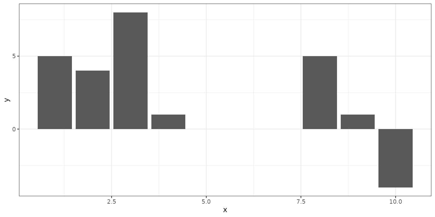
This does not look right…

You might have tried geom_bar() and gotten an error. geom_bar() counts the number of cases for each x in the data set and should not be supplied a y aesthetic mapping.

Individual geoms: geom_col()

p_xy + geom_col(
  position =
    position_dodge2(preserve = "single")
)

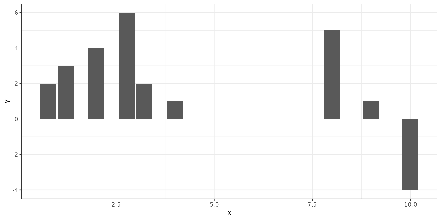
Default is position = "stack", this puts same x values on top of each other. Setting it to dodge separates overlapping values.

Collective geoms

p_xy + geom_line(aes(group = gr))

p_xy + geom_line(aes(linetype = gr))

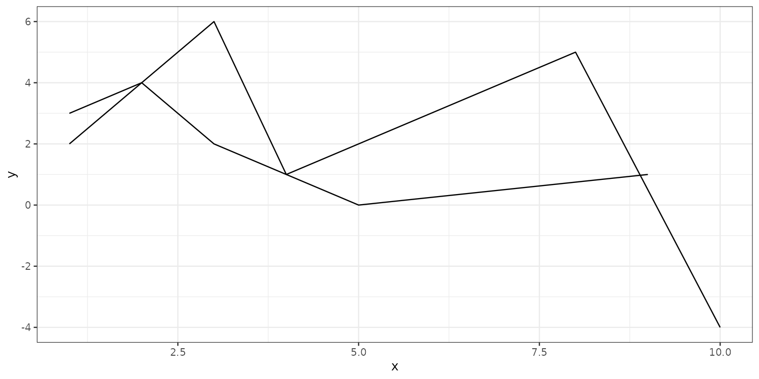
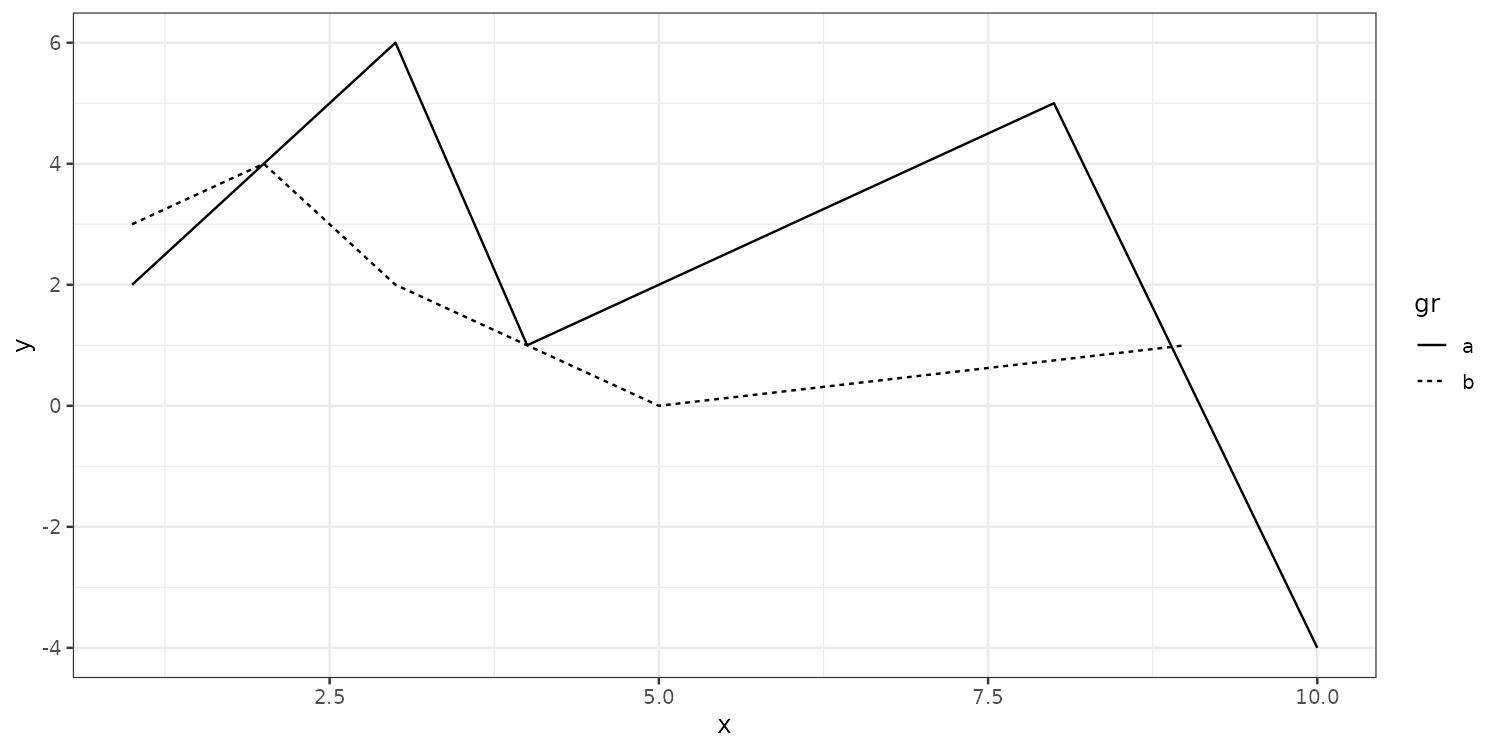
Collective geoms are plots with connected observations. group tells ggplot how to connect the data.

When assigning an aesthetic (color, fill, linetype, shape, size) to the group ggplot adds a legend.

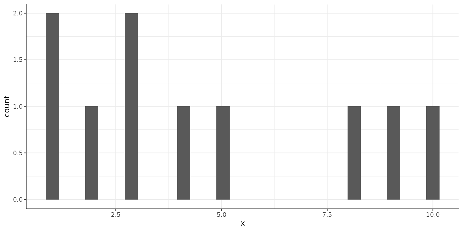
Statistical summaries: geom_histogram()

ggplot(data=df, aes(x=x)) +
  geom_histogram()

geom_histogram(), like geom_bar() and geom_density() counts x values. It would error if we supplied a y.

Statistical summaries: geom_smooth()

p_xy + geom_point() + geom_smooth()

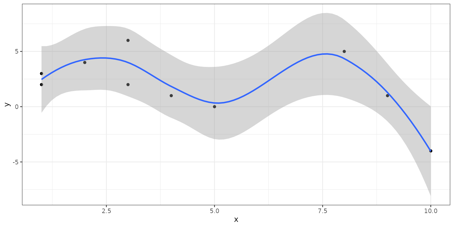
By default geom_smooth() fits a loess curve. Pass method = "lm" for a straight line.

Statistical summaries: geom_errorbar()

p_xy + geom_errorbar(aes(ymin = y - 1, ymax = y + 1))

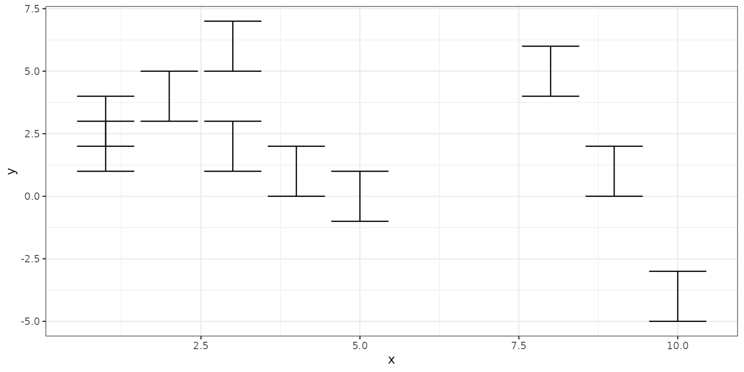
Useful for reporting e.g., coefficient plots, but requires ymin and ymax aesthetics.

Grouping and summarizing

• ggplot intro

• Plot types

• Grouping and summarizing

• Styling

• Wrapping up

Grouping and summarizing

What if we wanted to plot how GDP per capita has developed for each country over time. A line plot should do this well.

ggplot(
  gapminder_dt,
  aes(x = year,
      y = gdpPercap)
) +
  geom_line()

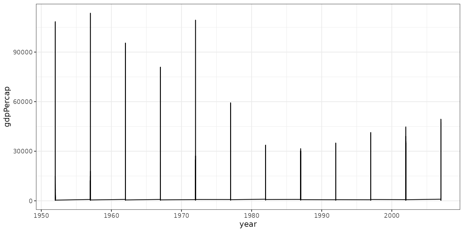
Any idea what’s wrong?

The group aesthetic

We need to tell ggplot to group the data by country.

ggplot(
  gapminder_dt,
  aes(x = year,
      y = gdpPercap,
      group = country)
) +
  geom_line()

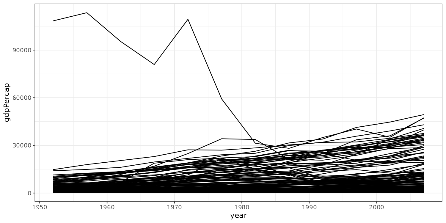
Still quite hard to see what’s going on!

Making things clearer

Let’s color lines by continent.

ggplot(
  gapminder_dt,
  aes(x = year,
      y = gdpPercap,
      group = country,
      color = continent)
) +
  geom_line()

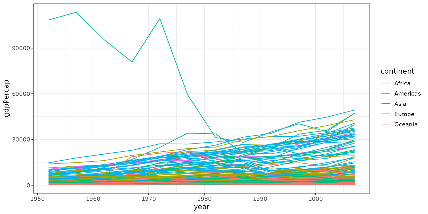
Still looks cluttered.

color sets the color of lines and points, fill configures color of areas, e.g. bar plots. And for you brits out there, colour is also allowed.

Faceting

Instead we could split the plot into subplots by continent.

ggplot(
  gapminder_dt,
  aes(x = year,
      y = gdpPercap,
      group = country)
) +
  geom_line() +
  facet_wrap(vars(continent))

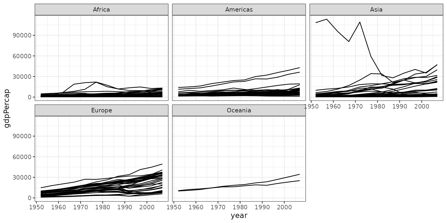
By default facet_wrap() keeps the x and y scales identical across panels. Pass scales = "free_y", "free_x", or "free" to let them vary.

Styling

• ggplot intro

• Plot types

• Grouping and summarizing

• Styling

• Wrapping up

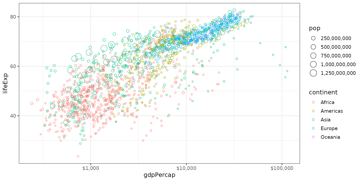
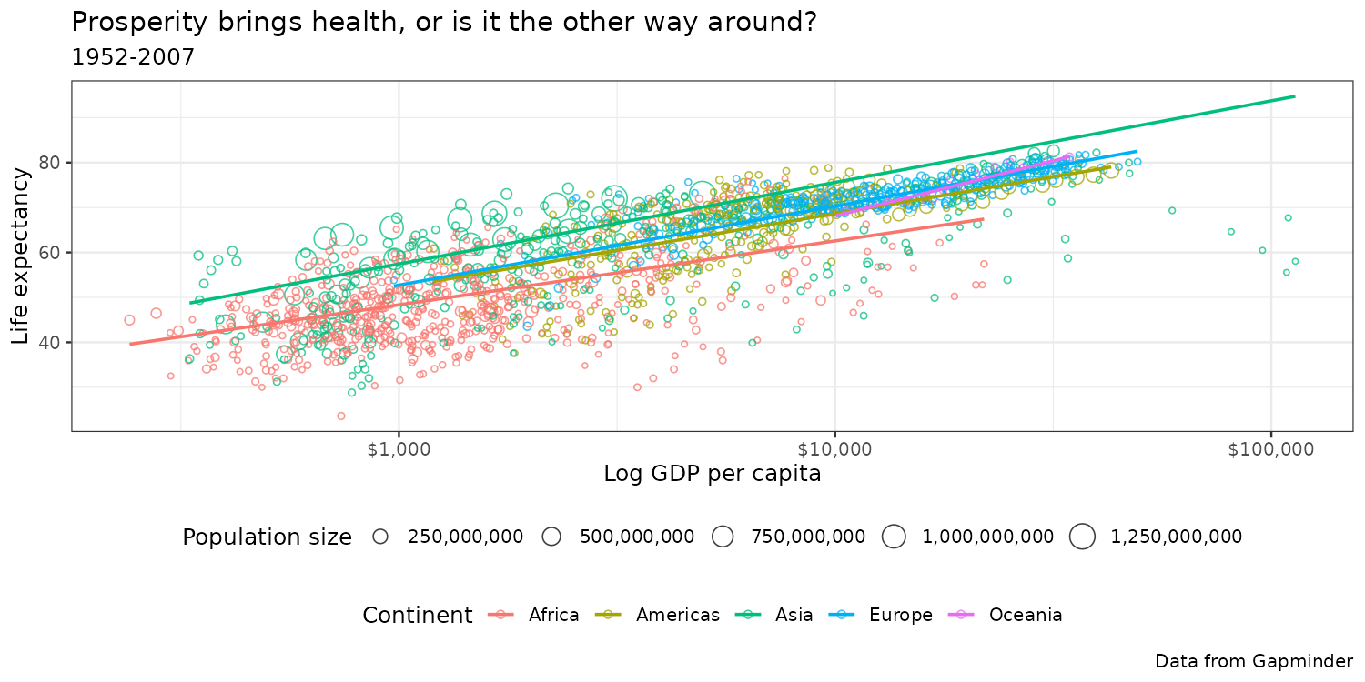
A plot to work on

p <- ggplot(
  gapminder_dt,
  aes(x = gdpPercap,
      y = lifeExp)
)
p + geom_point()

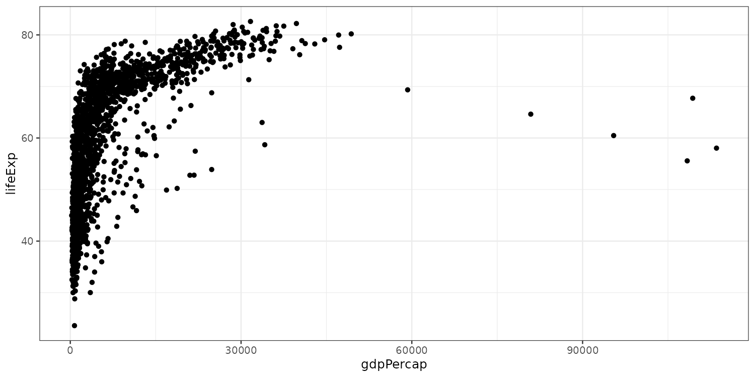
How can we increase readability?

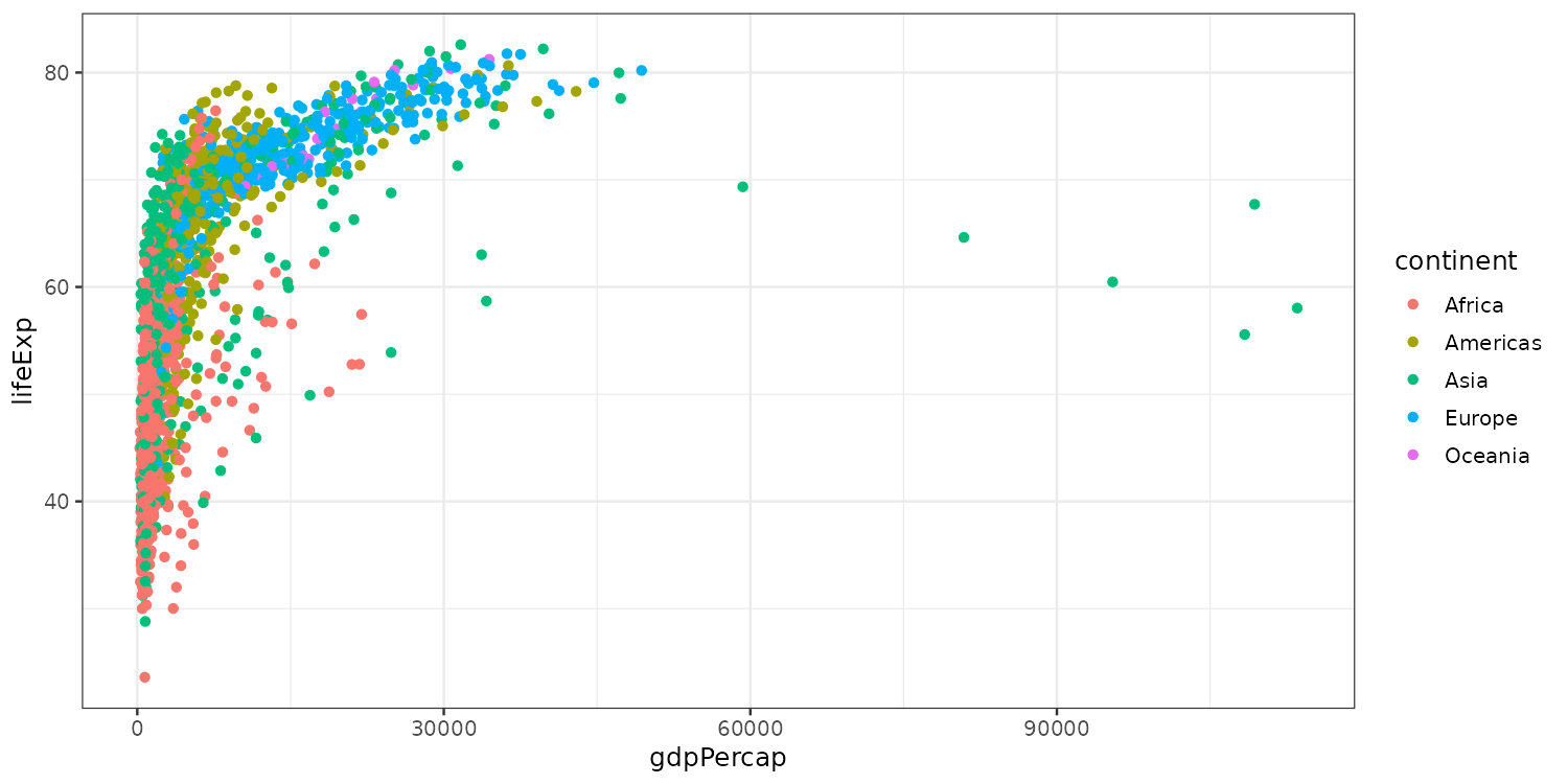
Configuring scales: color

ggplot(gapminder_dt,
       aes(x = gdpPercap,
           y = lifeExp)) +
  geom_point(aes(color = continent))

Configuring scales: size

ggplot(gapminder_dt,
       aes(x = gdpPercap,
           y = lifeExp)) +
  geom_point(aes(color = continent,
                 size = pop),
             shape = 1, alpha = 0.75) +
  scale_size(labels = scales::comma)

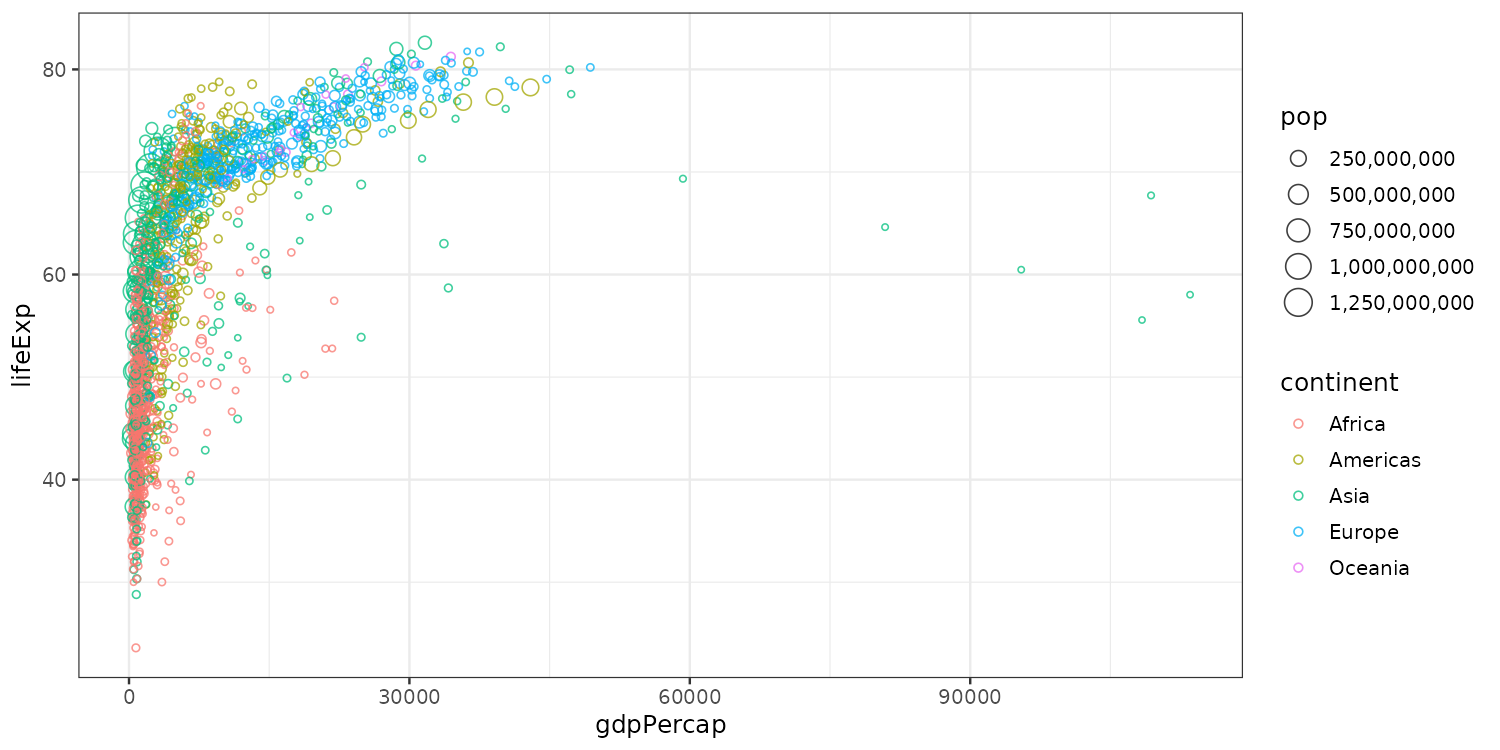
• Makes point size vary with population size,
• with semi-transparent hollow circles
• Change size scale to non-scientific

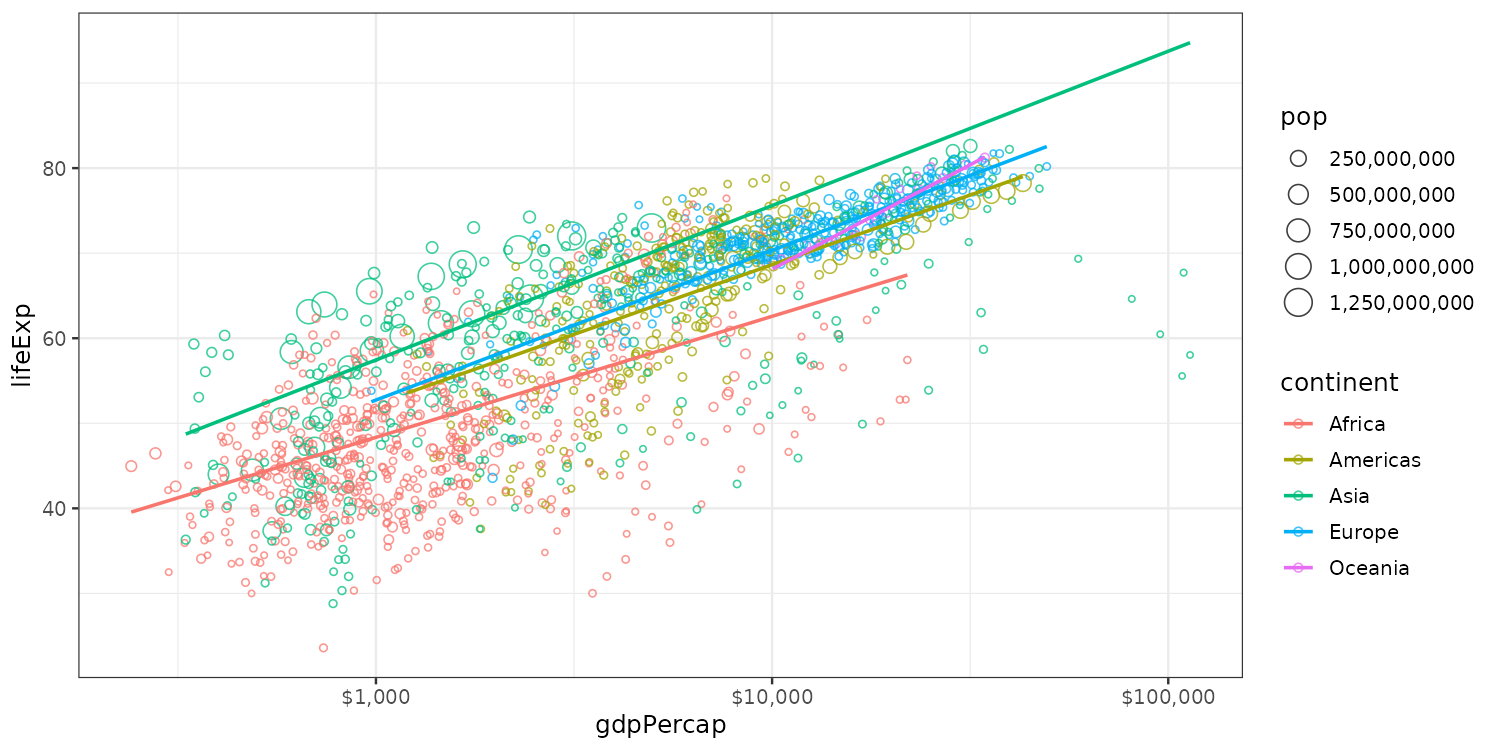
Configuring scales: logarithmic x-scale

ggplot(gapminder_dt,
       aes(x = gdpPercap,
           y = lifeExp)) +
  geom_point(aes(color = continent,
                 size = pop),
             shape = 1, alpha = 0.75) +
  scale_size(labels = scales::comma) +
  scale_x_log10(labels = scales::dollar)

scale_y_log10() is short for scale_y_continuous(transform = transform_log10()).

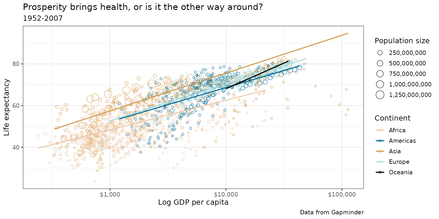
Adding (population weighted) regression lines

p <- ggplot(gapminder_dt,
       aes(x = gdpPercap,
           y = lifeExp,
           color = continent)) +
  geom_point(aes(size = pop),
             shape = 1, alpha = 0.75) +
  scale_size(labels = scales::comma) +
  scale_x_log10(labels = scales::dollar) +
  geom_smooth(aes(weight = pop),
              linewidth = 0.8,
              method = "lm", se = FALSE)
p

Note how I moved the color aesthetic to the main ggplot() call so it applies to both geoms.

Writing for the reader

A figure that needs explaining is half-finished. Titles, captions, and a line of narrative do the rest.

• Title: state the point, not the chart type. “Unemployment converged across municipalities” beats “Unemployment by year”.
• Subtitle: scope, e.g. “290 Swedish municipalities, 2016–2023”.
• Axis labels: human-readable, with units. No raw variable names.
• Caption: source, sample, and caveats the reader cannot infer from the panel.

Adding plot labels

p <- p +
  labs(
    x = "Log GDP per capita",
    y = "Life expectancy",
    color = "Continent",
    size = "Population size",
    title = "Prosperity brings health, or is it the other way around?",
    subtitle = "1952-2007",
    caption = "Data from Gapminder"
  )
p

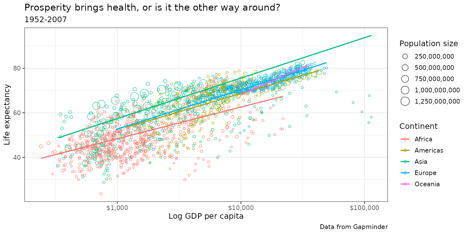
theme() sets look and feel

p + theme_bw() +
  theme(plot.title = element_text(size=16))

p + theme(legend.position = "bottom",
          legend.box = "vertical")

See ?theme for all the things you can edit!

Aside on colors: three palette types

• We do not perceive all colors the same.
• When plotting, try to use palettes designed for perceptual uniformity.
• Three types of palettes, depending on data structure:
  • Sequential: for ordered data (e.g., income)
  • Diverging: ordered with midpoint (correlation, temperature)
  • Qualitative: unordered, categorical, data (countries, species)

Color blindness: a simulator function

8% of men and 0.5% of women have some form of color blindness. Let’s create a function to evaluate how different palettes look for people who are color blind.

library(dichromat)
library(paletteer)
colorblind_palette = function(palette) {
  melt(as.data.table(
    append(
      list(x = seq_along(palette),
           "Trichromacy (Original)" = palette),
      lapply(c("Protanopia"="protan", "Deutanopia"="deutan", "Tritanopia"="tritan"),
             dichromat, colours = palette)
    )
  ), id.vars = "x") |>
    ggplot(aes(x=x, y = 0, fill = value)) +
    geom_raster() + facet_wrap(vars(variable), nrow=4) +
    scale_fill_identity() + theme_void() + theme(legend.position = "none")
}

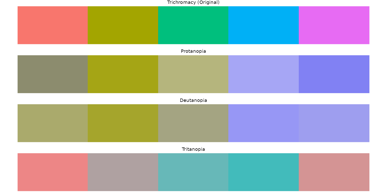
Color blindness: ggplot2 default hue

colorblind_palette(scales::hue_pal()(5))

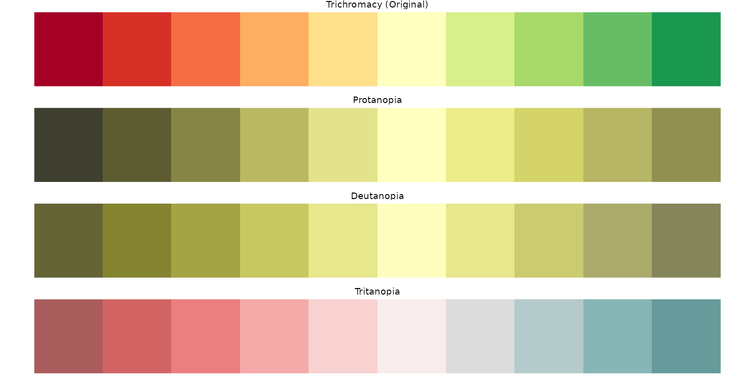
Color blindness: RColorBrewer RdYlGn

colorblind_palette(paletteer_d("RColorBrewer::RdYlGn", 10))

Color blindness: Wes Anderson Darjeeling 2

colorblind_palette(paletteer_d("wesanderson::Darjeeling2", 5))

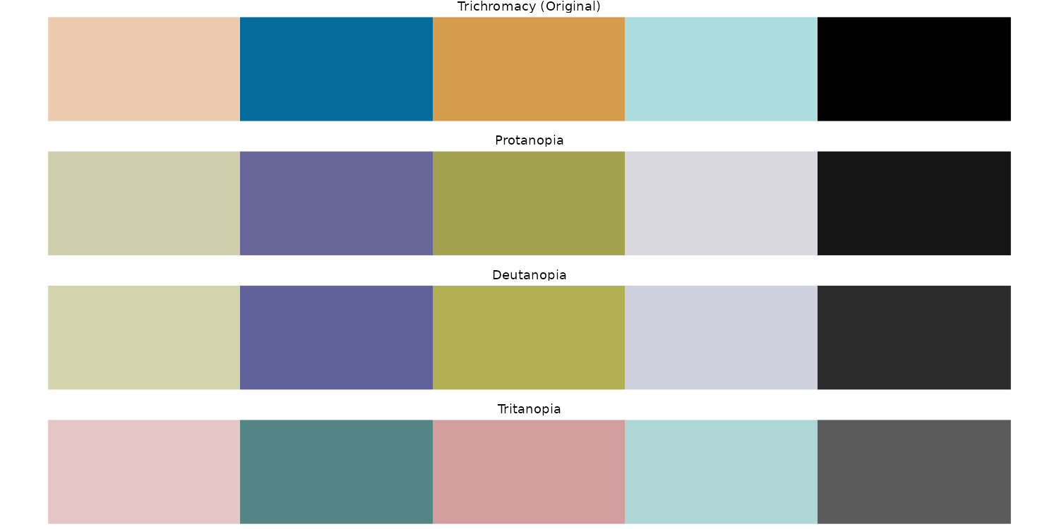
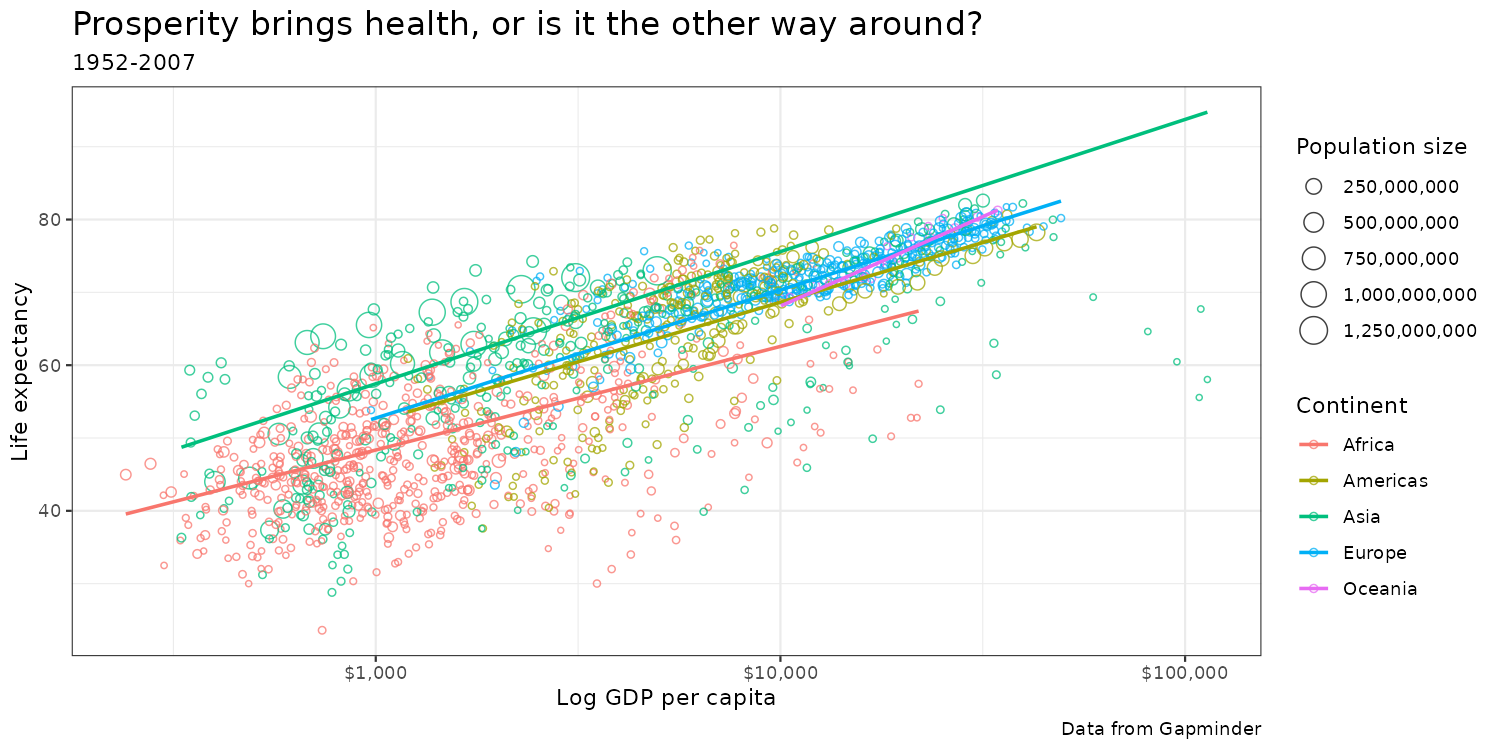
Let’s go with this one for our plot!

Final result

Saving figures with ggsave()

• It sounds easy, but saving a figure can quite messy, even if it looked great in the viewer.
• ggsave(<filename>, p) saves the p plot object to a file
• The file ending determines the graphics device:
  • Vector formats (.pdf, .svg) look much nicer
  • Raster formats (.png, .jpg) are easier to work with
• Use arguments width, height, and scale to get the size right

It can be quite hard to get custom fonts looking the way you want with vector formats. With rasterized formats the ragg package makes it super easy. For vectors, use svglite and make sure the font is installed on the system.

Wrapping up

• ggplot intro

• Plot types

• Grouping and summarizing

• Styling

• Wrapping up

Best practices

• Choose the right plot for your data and question
• Use labels to explain your plot
• Keep it clean, don’t plot too much on the same chart
• Use colors sparingly, effectively, accounting for colorblindness

Common pitfalls to avoid

• Misleading axes (bar charts not starting at zero 🫢)
• Overplotting (too much data)
• Chartjunk (prominent gridlines, backgrounds)
• 3D plots, pie charts (hard to read)

What changes, what doesn’t

Tools that will move fast before next year:

• IDE assistants and agents
• LLMs as data tools, not just as callers
• Visualization libraries (more interactive, more declarative)

Habits that move slowly:

• Knowing your data and its provenance
• Validating before trusting a number
• Asking the right question
• Communicating a result so someone else can act on it

LLMs as plot generators

I’ve been experimenting with gpt-image-2 to generate slide infographics. Image generation has gotten good enough to get text right, but representing data truthfully is still a challenge. Although it does generate beatiful figures with the right prompt.

Course arc, looking back

 

• Every block has the same shape: real data, a small toolkit, a validation step
• The tools will keep changing; the workflow shape does not

The end

• Written exam: Thursday, June 4, 2026, 08:00–11:00
• Re-exam: Friday, August 28, 2026
• Code reading, workflow judgment, debugging logic, data-source judgment — not syntax memorization
• Advice: lecture handouts include notes that could give useful context.
• Good luck!

Visualization Resources

• Data Visualization: A practical introduction by Kieran Healy
• Chapters 1,9,10 of R4DS
• The 3rd edition ggplot book (advanced, WIP)

References

Anscombe, F. J. 1973. “Graphs in Statistical Analysis.” The American Statistician, no. 27: 17–21.

Healy, Kieran. 2018. Data Visualization: A Practical Introduction. 1st edition. Princeton University Press.

Matejka, Justin, and George Fitzmaurice. 2017. “Same Stats, Different Graphs: Generating Datasets with Varied Appearance and Identical Statistics Through Simulated Annealing.” Proceedings of the 2017 CHI Conference on Human Factors in Computing Systems (New York, NY, USA), May 2, 1290–94. https://doi.org/10.1145/3025453.3025912.

Snow, John. 1855. On the Mode of Communication of Cholera. 2nd ed. John Churchill.

Tufte, Edward R. 1983. The Visual Display of Quantitative Information. 2nd ed. Graphics Press USA.

Wickham, Hadley, Mine Cetinkaya-Rundel, and Garrett Grolemund. 2023. R for Data Science: Import, Tidy, Transform, Visualize, and Model Data. 2nd edition. O’Reilly Media.